Learning objectives#
By the end you will be able to:
- Write a multiple regression model in matrix form \(\mathbf{y} = \mathbf{X}\boldsymbol{\beta} + \boldsymbol{\varepsilon}\) and build the design matrix, including the intercept column.
- Derive the normal equations \(\mathbf{X}^\top\mathbf{X}\hat{\boldsymbol{\beta}} = \mathbf{X}^\top\mathbf{y}\) and explain why libraries solve them with QR or SVD instead of an explicit inverse.
- Solve a three-parameter problem by hand and check it against NumPy, scikit-learn and statsmodels.
- Interpret a coefficient as a partial effect "holding the other features constant", and explain why it can change sign when features are added.
- Explain the difference between \(R^2\) and adjusted \(R^2\), and why neither replaces held-out validation.
- State the Gauss–Markov assumptions and run the matching diagnostics: residual plots, Breusch–Pagan, Q-Q, Durbin–Watson, VIF, leverage and Cook's distance.
- Implement batch gradient descent, explain why feature scaling decides whether it converges, and map scaled coefficients back to original units.
- Fit Ridge and Lasso in a leakage-safe scikit-learn
Pipeline, tune the penalty by cross-validation, and report the comparison honestly.
Prerequisites#
- The beginner tutorial: slope, intercept, residual, \(R^2\), RMSE.
- Linear algebra basics: matrix multiplication, transpose, inverse, rank. You do not need to have proved anything; you need to be able to read \(\mathbf{X}^\top\mathbf{X}\) and know it is a square matrix.
- Calculus at the level of "set the derivative to zero to find a minimum".
- Python 3.10 or newer and
pip. Comfortable running a script from a terminal.
Setup (all labs)#
mkdir -p ~/lr-expert-labs && cd ~/lr-expert-labs
python3 -m venv .venv
source .venv/bin/activate            # Windows PowerShell: .venv\Scripts\Activate.ps1
pip install --upgrade pip
pip install numpy scipy pandas scikit-learn statsmodels matplotlib
python -c "import numpy, sklearn, statsmodels; print(numpy.__version__, sklearn.__version__, statsmodels.__version__)"
The reference run for this page used Python 3.13.5 with numpy 2.5.3, scipy 1.18.1, pandas 3.0.6, scikit-learn 1.9.1, statsmodels 0.15.0 and matplotlib 3.11.2. Everything runs locally and offline after the install; no cloud account is needed.
Download all lab scripts and expected outputs (zip) linreg-expert-labs.zip · 10 files · 11 KB
1. The multiple linear regression model#
With \(p\) features, each observation \(i\) is modelled as
| Symbol | Meaning |
|---|---|
| \(n\) | Number of observations (rows) |
| \(p\) | Number of features, not counting the intercept |
| \(y_i\) | Target value for row \(i\) |
| \(x_{ij}\) | Value of feature \(j\) in row \(i\) |
| \(\beta_0\) | Intercept: expected \(y\) when every feature equals 0 |
| \(\beta_j\) | Partial slope of feature \(j\): change in expected \(y\) for a one-unit increase in \(x_j\), holding all other features in the model fixed |
| \(\varepsilon_i\) | Unobserved error: everything about \(y_i\) the features do not capture |
"Linear" means linear in the parameters \(\beta\), not in the raw inputs. \(y = \beta_0 + \beta_1 x + \beta_2 x^2 + \beta_3 \log z + \varepsilon\) is still a linear regression model, because each \(\beta\) multiplies a known column.
Matrix form and the design matrix#
Stack the \(n\) equations into one:
| Symbol | Shape | Meaning |
|---|---|---|
| \(\mathbf{y}\) | \(n \times 1\) | Target vector |
| \(\mathbf{X}\) | \(n \times (p+1)\) | Design matrix: one row per observation, one column per parameter |
| first column of \(\mathbf{X}\) | \(n \times 1\) | All ones: the intercept column. Multiplying it by \(\beta_0\) adds the same constant to every prediction |
| \(\boldsymbol{\beta}\) | \((p+1) \times 1\) | Coefficient vector, intercept first |
| \(\boldsymbol{\varepsilon}\) | \(n \times 1\) | Error vector |
A hat means "estimated from data": \(\hat{\boldsymbol{\beta}}\) are the fitted coefficients, \(\hat{\mathbf{y}} = \mathbf{X}\hat{\boldsymbol{\beta}}\) the fitted values, \(\mathbf{e} = \mathbf{y} - \hat{\mathbf{y}}\) the residuals.
Libraries disagree on who adds the intercept column. This causes real bugs:
| Tool | Adds the intercept automatically? |
|---|---|
sklearn.linear_model.LinearRegression |
Yes (fit_intercept=True by default) |
statsmodels.api.OLS |
No: call sm.add_constant(X) first |
statsmodels.formula.api.ols("y ~ x1 + x2", df) |
Yes |
np.linalg.lstsq(X, y) |
No: you build the column yourself |
2. OLS derivation: from squared error to the normal equations#
For a candidate \(\boldsymbol{\beta}\), the residual vector is \(\mathbf{y} - \mathbf{X}\boldsymbol{\beta}\). OLS minimises the residual sum of squares:
- \(S(\boldsymbol{\beta})\) is the sum of squared residuals for that choice of coefficients: the same quantity the beginner page minimised, now for all features at once.
- \(\lVert \mathbf{v} \rVert^2\) is the sum of squared entries of a vector \(\mathbf{v}\), which equals \(\mathbf{v}^\top\mathbf{v}\).
- \(^\top\) is the transpose. The two cross terms \(\mathbf{y}^\top\mathbf{X}\boldsymbol{\beta}\) and \(\boldsymbol{\beta}^\top\mathbf{X}^\top\mathbf{y}\) are the same scalar, so they combine into \(2\boldsymbol{\beta}^\top\mathbf{X}^\top\mathbf{y}\).
Take the gradient with respect to \(\boldsymbol{\beta}\), using \(\partial(\boldsymbol{\beta}^\top\mathbf{a})/\partial\boldsymbol{\beta} = \mathbf{a}\) and \(\partial(\boldsymbol{\beta}^\top\mathbf{A}\boldsymbol{\beta})/\partial\boldsymbol{\beta} = 2\mathbf{A}\boldsymbol{\beta}\) for a symmetric matrix \(\mathbf{A}\):
- \(\nabla S\) is the vector of partial derivatives of \(S\), one per coefficient.
- \(\mathbf{X}^\top\mathbf{X}\) is a \((p+1) \times (p+1)\) symmetric matrix of sums of products of columns; \(\mathbf{X}^\top\mathbf{y}\) is a \((p+1) \times 1\) vector of sums of products of each column with \(y\).
Set the gradient to zero:
- The left equation is the normal equations: \(p+1\) linear equations in \(p+1\) unknowns.
- \(\hat{\boldsymbol{\beta}}\) is the OLS estimate.
- \((\mathbf{X}^\top\mathbf{X})^{-1}\) is the inverse of \(\mathbf{X}^\top\mathbf{X}\). The closed form on the right is valid only when that inverse exists.
Why this is a minimum. The Hessian is \(\nabla^2 S = 2\mathbf{X}^\top\mathbf{X}\). For any vector \(\mathbf{v}\), \(\mathbf{v}^\top\mathbf{X}^\top\mathbf{X}\mathbf{v} = \lVert \mathbf{X}\mathbf{v} \rVert^2 \ge 0\), so the Hessian is positive semi-definite and \(S\) is convex. If \(\mathbf{X}\) has full column rank (\(\operatorname{rank}(\mathbf{X}) = p+1\)), \(\mathbf{X}^\top\mathbf{X}\) is positive definite and the minimiser is unique.
When \(\mathbf{X}^\top\mathbf{X}\) is not invertible. If one column is an exact linear combination of others (all one-hot dummies plus an intercept, the same quantity in two units), or if \(p + 1 > n\), then \(\operatorname{rank}(\mathbf{X}) < p+1\), \(\mathbf{X}^\top\mathbf{X}\) is singular, and infinitely many \(\boldsymbol{\beta}\) reach the same minimum. The usual fixes: remove the redundant column, take the minimum-norm solution from the pseudo-inverse, or regularise with Ridge (Section 10).
Two facts that hold for every OLS fit (they follow from the normal equations; they are not assumptions):
- \(\mathbf{e} = \mathbf{y} - \mathbf{X}\hat{\boldsymbol{\beta}}\) is the residual vector. The first equation says residuals are orthogonal to every column of \(\mathbf{X}\).
- The first row of that equation, for the column of ones, gives \(\sum e_i = 0\). The fitted plane passes through the point of means \((\bar{x}_1, \ldots, \bar{x}_p, \bar{y})\).
3. Geometry, the hat matrix, and why nobody inverts \(\mathbf{X}^\top\mathbf{X}\)#
Think of \(\mathbf{y}\) as a point in \(n\)-dimensional space. Every possible prediction \(\mathbf{X}\boldsymbol{\beta}\) lies in the column space of \(\mathbf{X}\), a \((p+1)\)-dimensional subspace. OLS picks the point in that subspace closest to \(\mathbf{y}\): the orthogonal projection.
- \(\mathbf{H} = \mathbf{X}(\mathbf{X}^\top\mathbf{X})^{-1}\mathbf{X}^\top\) is the \(n \times n\) hat matrix ("it puts the hat on \(\mathbf{y}\)").
- \(\mathbf{I}\) is the \(n \times n\) identity matrix; \(\mathbf{I} - \mathbf{H}\) is the "residual maker".
| Property | Statement | Meaning |
|---|---|---|
| Symmetric | \(\mathbf{H}^\top = \mathbf{H}\) | Orthogonal (not oblique) projection |
| Idempotent | \(\mathbf{H}\mathbf{H} = \mathbf{H}\) | Projecting twice changes nothing |
| Trace | \(\operatorname{trace}(\mathbf{H}) = p+1\) | Equals the number of fitted parameters |
| Leverage | \(h_{ii}\) = diagonal entry \(i\), with \(0 \le h_{ii} \le 1\) | How strongly \(y_i\) pulls its own fitted value \(\hat{y}_i\) |
| Average leverage | \(\frac{1}{n}\sum h_{ii} = (p+1)/n\) | Baseline for "high leverage" rules of thumb |
Pythagoras in this geometry gives the variance decomposition used by \(R^2\) (with an intercept in the model):
- \(\mathbf{1}\) is a vector of ones and \(\bar{y}\) the mean of \(y\).
- \(\mathrm{SS_{tot}}\) is total variation of \(y\) around its mean, \(\mathrm{SS_{reg}}\) the part captured by the fitted values, \(\mathrm{SS_{res}}\) the part left in the residuals.
Numerics: QR and SVD instead of an inverse#
The formula \((\mathbf{X}^\top\mathbf{X})^{-1}\mathbf{X}^\top\mathbf{y}\) is for derivation and hand work. Numerical code avoids it, mainly because forming \(\mathbf{X}^\top\mathbf{X}\) squares the condition number:
- \(\kappa\) is the 2-norm condition number, the ratio of the largest to the smallest singular value \(\sigma\). It measures how much small changes in the data can move the solution.
- Double precision carries about 16 significant digits; roughly \(\log_{10}\kappa\) of them can be lost. In Lab 1, a nearly collinear design has \(\kappa(\mathbf{X}) \approx 2.089 \times 10^6\) and \(\kappa(\mathbf{X}^\top\mathbf{X}) \approx 4.358 \times 10^{12}\): only about four reliable digits remain once you form \(\mathbf{X}^\top\mathbf{X}\).
| Method | What it does | When |
|---|---|---|
| QR | Factor \(\mathbf{X} = \mathbf{Q}\mathbf{R}\) (orthonormal \(\mathbf{Q}\), upper-triangular \(\mathbf{R}\)), then solve \(\mathbf{R}\hat{\boldsymbol{\beta}} = \mathbf{Q}^\top\mathbf{y}\) by back-substitution | Standard for full-rank problems; error depends on \(\kappa(\mathbf{X})\), not its square |
| SVD | Factor \(\mathbf{X} = \mathbf{U}\boldsymbol{\Sigma}\mathbf{V}^\top\), then \(\hat{\boldsymbol{\beta}} = \mathbf{V}\boldsymbol{\Sigma}^{+}\mathbf{U}^\top\mathbf{y}\) | Most robust; handles rank deficiency and returns the minimum-norm solution. np.linalg.lstsq uses an SVD-based LAPACK routine (gelsd) |
| Pseudo-inverse | \(\hat{\boldsymbol{\beta}} = \mathbf{X}^{+}\mathbf{y}\) via np.linalg.pinv |
Same answer as the SVD route; use when you need the matrix itself |
| Cholesky on \(\mathbf{X}^\top\mathbf{X}\) | Factor \(\mathbf{X}^\top\mathbf{X} = \mathbf{L}\mathbf{L}^\top\), two triangular solves | Fast for very tall, well-conditioned data; inherits the squared condition number |
| Iterative (GD, SGD, conjugate gradient) | Step towards the minimum | Data too large for memory, or streaming (Section 9) |
scikit-learn's LinearRegression solves dense problems with SciPy's lstsq, so it does not form an explicit inverse either. Lab 1 shows six routes (inverse, solve, lstsq, QR, pinv, scikit-learn) agreeing to about \(10^{-15}\) on well-conditioned data.
4. Inference: standard errors, t-tests, intervals and the F-test#
Coefficients alone do not tell you how precisely they are estimated. Under the Gauss–Markov assumptions (Section 8), and with normal errors for exact small-sample results:
- \(\sigma^2\) is the true error variance and \(\hat{\sigma}^2\) its unbiased estimate. \(n - p - 1\) is the residual degrees of freedom: rows minus fitted parameters.
- \(\big[(\mathbf{X}^\top\mathbf{X})^{-1}\big]_{jj}\) is the \(j\)-th diagonal entry of the inverse.
- \(\operatorname{SE}(\hat{\beta}_j)\) is the standard error: the estimated standard deviation of \(\hat{\beta}_j\) across repeated samples.
- \(t_j\) tests \(H_0: \beta_j = 0\) against a t distribution with \(n - p - 1\) degrees of freedom.
- \(t_{1-\alpha/2,\, n-p-1}\) is the critical value; for a 95% interval \(\alpha = 0.05\).
- The p-value is the probability, if \(H_0\) and the model assumptions hold, of a t statistic at least as extreme as the one observed. It is not the probability that \(H_0\) is true, and a large p-value is not evidence that \(\beta_j = 0\).
At a new point \(\mathbf{x}_0\) (a row vector with a leading 1):
- The first is a confidence interval for the average \(y\) at \(\mathbf{x}_0\). The second is a prediction interval for one new observation; the extra 1 adds the irreducible noise \(\sigma^2\), so it is always wider.
The overall F-test asks whether all slopes are jointly zero (\(H_0: \beta_1 = \cdots = \beta_p = 0\)):
- \(p\) and \(n - p - 1\) are the numerator and denominator degrees of freedom.
5. Worked example (a): multiple regression by hand#
Caveat: made-up data. This example uses six synthetic rows designed for hand calculation. With 3 parameters there are only 3 residual degrees of freedom, so the p-values and intervals below illustrate the mechanics only. Do not read them as evidence about real cloud bills.
Setting. Monthly cloud bill \(y\) (in units of $100) for six teams, explained by \(x_1\) = number of VMs and \(x_2\) = storage in TB.
| Row | \(x_1\) (VMs) | \(x_2\) (TB) | \(y\) (bill, $100s) |
|---|---|---|---|
| 1 | 1 | 2 | 5 |
| 2 | 2 | 1 | 7 |
| 3 | 3 | 3 | 12 |
| 4 | 4 | 3 | 13 |
| 5 | 5 | 5 | 19 |
| 6 | 6 | 4 | 19 |
\(n = 6\), \(p = 2\). The correlation between \(x_1\) and \(x_2\) is 0.8315: related, not duplicates.
Step 1: design matrix#
The first column is the intercept column, the second is \(x_1\), the third is \(x_2\).
Step 2: \(\mathbf{X}^\top\mathbf{X}\)#
Each entry is a sum:
- \(\sum x_1 = 21\), \(\sum x_2 = 18\), \(\sum x_1^2 = 91\), \(\sum x_2^2 = 64\), and \(\sum x_1x_2 = 2+2+9+12+25+24 = 74\).
Step 3: \((\mathbf{X}^\top\mathbf{X})^{-1}\) via determinant and adjugate#
- \(\det\) is the determinant; a non-zero value confirms the matrix is invertible.
- \(\operatorname{adj}\) is the adjugate (transpose of the cofactor matrix). For a \(3 \times 3\) matrix, inverse = adjugate / determinant.
Step 4: \(\mathbf{X}^\top\mathbf{y}\)#
- \(\sum x_1 y = 5+14+36+52+95+114 = 316\) and \(\sum x_2 y = 10+7+36+39+95+76 = 263\).
Step 5: \(\hat{\boldsymbol{\beta}} = (\mathbf{X}^\top\mathbf{X})^{-1}\mathbf{X}^\top\mathbf{y}\)#
First \(\operatorname{adj}(\mathbf{X}^\top\mathbf{X})\,\mathbf{X}^\top\mathbf{y} = [216,\; 702,\; 459]^\top\) (for example \(348 \cdot 75 - 12 \cdot 316 - 84 \cdot 263 = 216\)). Divide by 324:
Fitted model:
- Holding storage constant, each extra VM is associated with about 2.1667 more on the predicted bill ($216.67).
- Holding the VM count constant, each extra TB is associated with about 1.4167 more ($141.67).
- The intercept 0.6667 ($66.67) is the prediction at 0 VMs and 0 TB. That point lies outside the data, so treat it as a mathematical anchor, not an estimate of a real fixed fee.
Step 6: predictions, residuals, leverage, Cook's distance#
| Row | \(y\) | \(\hat{y}\) (exact) | \(\hat{y}\) | \(e = y - \hat{y}\) | leverage \(h_{ii}\) | Cook's \(D_i\) |
|---|---|---|---|---|---|---|
| 1 | 5 | 17/3 | 5.6667 | −0.6667 | 0.6296 | 1.1657 |
| 2 | 7 | 77/12 | 6.4167 | +0.5833 | 0.6574 | 1.0891 |
| 3 | 12 | 137/12 | 11.4167 | +0.5833 | 0.2130 | 0.0669 |
| 4 | 13 | 163/12 | 13.5833 | −0.5833 | 0.2130 | 0.0669 |
| 5 | 19 | 223/12 | 18.5833 | +0.4167 | 0.6574 | 0.5557 |
| 6 | 19 | 58/3 | 19.3333 | −0.3333 | 0.6296 | 0.2914 |
Checks: \(\sum e_i = 0\) and \(\mathbf{X}^\top\mathbf{e} = [0, 0, 0]^\top\) exactly; \(\sum h_{ii} = 3 = p + 1\). Leverage and Cook's distance are explained in Section 8.
Step 7: sums of squares, \(R^2\), adjusted \(R^2\), RMSE#
- \(169.75 + 1.75 = 171.5\) confirms \(\mathrm{SS_{tot}} = \mathrm{SS_{reg}} + \mathrm{SS_{res}}\).
- RMSE uses \(\sqrt{\mathrm{SS_{res}}/n}\), the same convention as the beginner page. In dollars it is about $54.01; MAE is the mean absolute residual.
Step 8: inference (verified with statsmodels)#
\(\hat{\sigma}^2 = 1.75/3 = 7/12 \approx 0.5833\), so \(\hat{\sigma} \approx 0.7638\). With \(t_{0.975,\,3} = 3.1824\):
| Coefficient | Estimate | SE | t | p-value (df = 3) | 95% CI |
|---|---|---|---|---|---|
| \(\beta_0\) (intercept) | 0.6667 | 0.7915 | 0.842 | 0.4615 | [−1.8524, 3.1857] |
| \(\beta_1\) (VMs) | 2.1667 | 0.3287 | 6.592 | 0.0071 | [1.1207, 3.2126] |
| \(\beta_2\) (TB) | 1.4167 | 0.4348 | 3.258 | 0.0472 | [0.0330, 2.8004] |
Overall \(F = (169.75/2)/(1.75/3) = 145.5\) with (2, 3) degrees of freedom, p ≈ 0.00103.
Prediction at \(x_1 = 4,\ x_2 = 4\): \(\hat{y} = 2/3 + 4 \cdot 13/6 + 4 \cdot 17/12 = 15.0\). 95% confidence interval for the mean: [13.5967, 16.4033]. 95% prediction interval for one new team: [12.1933, 17.8067].
Caveat: illustration only. The p-value 0.0472 for storage sits just under 0.05 with 3 residual degrees of freedom; a small change to one row could move it to either side. Rows 1 and 2 have Cook's D above 1 because they sit at the edge of the feature space (leverage 0.63–0.66 against an average of 3/6 = 0.5). With six rows almost every point is influential. This is a hand-computation example, not a model to deploy.
6. Interpreting coefficients in multiple regression#
- \(\hat{\beta}_j\) is a partial effect: the change in expected \(y\) per unit of \(x_j\) with the other included features held fixed.
- It depends on which other features are in the model. Fit Example (a) with \(x_1\) alone and the slope is 3.0571 (\(R^2 = 0.9537\)), not 2.1667. Without \(x_2\) in the model, the VM coefficient absorbs part of the storage effect, because teams with more VMs also tend to store more. Adding a correlated feature can change a coefficient's size and even its sign.
- Frisch–Waugh–Lovell theorem. \(\hat{\beta}_j\) from the full regression equals the slope from regressing (residuals of \(y\) on the other features) on (residuals of \(x_j\) on the other features). Only the part of \(x_j\) not linearly explained by the others is used. That is the precise meaning of "holding others constant".
- Coefficients carry units (\(y\) per unit of \(x_j\)), so raw magnitudes are not comparable across features. Standardise first if you want "per standard deviation" effects, and remember collinearity makes individual magnitudes unstable.
- A coefficient is an association in observational data. It is a causal effect only under extra assumptions: no omitted confounders, correct functional form, no reverse causality.
Categorical features and the dummy variable trap#
A categorical feature with \(k\) levels (for example region east / north / south / west) becomes \(k\) indicator columns. With an intercept, the \(k\) indicators sum to the intercept column in every row, so \(\mathbf{X}\) is exactly collinear. In a verified 8-row example (intercept, one numeric feature, all 4 region dummies, so 6 columns), \(\operatorname{rank}(\mathbf{X}) = 5\) and \(\kappa(\mathbf{X}^\top\mathbf{X}) \approx 1.5 \times 10^{17}\): singular to machine precision.
Fix: use \(k - 1\) dummies (pd.get_dummies(..., drop_first=True) or OneHotEncoder(drop="first")). The dropped level is the reference; each remaining coefficient is the expected difference from it, holding other features fixed. With Ridge or Lasso, keeping all \(k\) is common because the penalty makes the solution unique. At prediction time, handle unseen levels explicitly (OneHotEncoder(handle_unknown="ignore")).
Interactions and polynomial terms#
- \(\beta_3\) is the interaction coefficient: the effect of \(x_1\) now depends on the value of \(x_2\).
- \(\mathbb{E}[y]\) is the expected value of \(y\) given the features. \(\beta_1\) alone is the effect of \(x_1\) only where \(x_2 = 0\). Centring both features before multiplying makes \(\beta_1\) the effect at the mean of \(x_2\) and usually reduces collinearity.
Polynomial terms (\(x, x^2, x^3\)) work the same way: curved in \(x\), linear in \(\beta\). Raw powers are highly correlated (centre them or use orthogonal polynomials), high degrees overfit and extrapolate badly, and if you keep \(x^2\) or \(x_1x_2\), keep the lower-order terms too. In scikit-learn, PolynomialFeatures(degree=2, include_bias=False) inside a Pipeline generates them.
7. \(R^2\) vs adjusted \(R^2\)#
- \(R^2\) is the fraction of the variation in \(y\) the model explains on the data evaluated.
- \(R^2_{\text{adj}}\) multiplies the unexplained fraction \(1 - R^2\) by \((n-1)/(n-p-1)\), a factor that grows with the number of features \(p\).
| Property | \(R^2\) | Adjusted \(R^2\) |
|---|---|---|
| Adding a feature (in-sample OLS with intercept) | Never decreases | Rises only if the new feature's \(\lvert t \rvert > 1\); otherwise falls |
| Range on training data | 0 to 1 | Can be negative |
| Example (a) | 97/98 ≈ 0.9898 | 289/294 ≈ 0.9830 |
| Use | Describe fit | Rough in-sample comparison of models with different \(p\) |
A verified demonstration: 30 synthetic rows with one real feature give \(R^2 = 0.6866\), adjusted 0.6754. Add five pure-noise features and \(R^2\) rises to 0.7179 while adjusted \(R^2\) falls to 0.6443. The noise raised \(R^2\) and made the model worse.
Two more points that matter in practice:
- Test-set \(R^2\) can be negative.
sklearn.metrics.r2_scoreon held-out data uses the test mean in \(\mathrm{SS_{tot}}\); a negative value means the model is worse than predicting that constant. - Neither replaces validation. Adjusted \(R^2\) is an in-sample correction. For any claim about prediction, use cross-validation or a held-out test set, as in Lab 3.
RMSE \(= \sqrt{\mathrm{SS_{res}}/n}\) and the residual standard error \(\hat{\sigma} = \sqrt{\mathrm{SS_{res}}/(n-p-1)}\) (what statsmodels and R report) differ only by the degrees-of-freedom correction. Say which one you quote.
8. Assumptions and diagnostics#
Gauss–Markov assumptions#
| # | Assumption | Formal statement |
|---|---|---|
| GM1 | Linear in parameters | \(\mathbf{y} = \mathbf{X}\boldsymbol{\beta} + \boldsymbol{\varepsilon}\) |
| GM2 | Full column rank (no perfect multicollinearity) | \(\operatorname{rank}(\mathbf{X}) = p + 1\) |
| GM3 | Strict exogeneity | \(\mathbb{E}[\boldsymbol{\varepsilon} \mid \mathbf{X}] = \mathbf{0}\) |
| GM4 | Spherical errors (homoscedastic, uncorrelated) | \(\operatorname{Var}(\boldsymbol{\varepsilon} \mid \mathbf{X}) = \sigma^2\mathbf{I}\) |
Gauss–Markov theorem: under GM1–GM4, OLS is BLUE, the Best Linear Unbiased Estimator. Among estimators that are linear in \(\mathbf{y}\) and unbiased, it has the smallest variance.
- Unbiasedness needs only GM1–GM3: \(\mathbb{E}[\hat{\boldsymbol{\beta}} \mid \mathbf{X}] = \boldsymbol{\beta} + (\mathbf{X}^\top\mathbf{X})^{-1}\mathbf{X}^\top\mathbb{E}[\boldsymbol{\varepsilon} \mid \mathbf{X}] = \boldsymbol{\beta}\).
- Normality is not a Gauss–Markov assumption. It makes t and F statistics exactly t- and F-distributed in small samples. With large \(n\), inference is approximately valid without it, provided GM1–GM4 hold.
- If GM4 fails, OLS stays unbiased but is no longer "best", and the classical \(\sigma^2(\mathbf{X}^\top\mathbf{X})^{-1}\) gives wrong standard errors.
- If GM3 fails (omitted confounder, measurement error in \(\mathbf{X}\), reverse causality), OLS is biased. Residual diagnostics alone cannot fully detect this.
- BLUE does not mean lowest mean squared error. Ridge is biased and can still have lower MSE (Section 10).
Caveat: thresholds are rules of thumb. The cut-offs below (VIF > 5 or > 10, condition number > 30 on scaled columns, Cook's D > 1 or > 4/n, leverage > 2(p+1)/n, Durbin–Watson roughly 1.5–2.5) are screening conventions, not hard limits. Use them to decide what to look at, then judge the practical consequence for your purpose. Plots first, tests second.
| Check | Tool | Common rule of thumb |
|---|---|---|
| Non-linearity | Residuals vs fitted, vs each feature | Visible curve: add terms or transform |
| Heteroscedasticity | Funnel in residual plot; Breusch–Pagan, White | Small p (for example < 0.05) suggests non-constant variance |
| Normality | Q-Q plot; Jarque–Bera; Shapiro–Wilk | Matters mainly for small-\(n\) inference and prediction intervals |
| Autocorrelation | Durbin–Watson (time-ordered data); Breusch–Godfrey | About 2 = none; below about 1.5 or above 2.5 worth investigating |
| Multicollinearity | VIF | > 5 deserves attention; > 10 often treated as serious |
| Conditioning | Condition number of standardised \(\mathbf{X}\) | > 30 often cited (Belsley, Kuh and Welsch) |
| Leverage | \(h_{ii}\) | > \(2(p+1)/n\) (or \(3(p+1)/n\)) |
| Influence | Cook's distance | > 1 large; > \(4/n\) worth a look |
| Outliers in \(y\) | Studentised residuals | \(\lvert r_i \rvert\) > 2 (or 3) worth a look |
Residual plots#
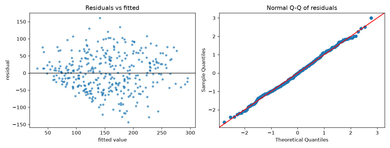
Figure 1. Lab 3 diagnostics on the diabetes training set (353 rows). Left: residuals form a band from roughly −150 to +160 around zero with no strong curve. Right: residual quantiles lie close to the 45° line.
- Residuals vs fitted should be a structureless band around 0. A curve suggests a missing non-linear term or interaction; a funnel suggests heteroscedasticity.
- Residuals vs each feature (including features not in the model) reveals mis-specification.
- Residuals vs time or row order: waves or runs indicate autocorrelation.
- Prefer studentised residuals \(r_i = e_i / \big(\hat{\sigma}\sqrt{1 - h_{ii}}\big)\), because \(\operatorname{Var}(e_i) = \sigma^2(1 - h_{ii})\): raw residuals at high-leverage points are naturally smaller.
Heteroscedasticity and Breusch–Pagan#
Heteroscedasticity means \(\operatorname{Var}(\varepsilon_i \mid \mathbf{X})\) changes across rows. The Breusch–Pagan test regresses the squared residuals \(e_i^2\) on the features:
- \(\mathrm{LM}\) is the Lagrange-multiplier test statistic; \(R^2_{\text{aux}}\) is the \(R^2\) of that auxiliary regression; \(\chi^2_p\) is the chi-squared distribution with \(p\) degrees of freedom. A small p-value is evidence of non-constant variance.
Remedies: heteroscedasticity-consistent ("robust", "sandwich") standard errors such as HC3 (fit(cov_type="HC3") in statsmodels), a variance-stabilising transform of \(y\) such as a log, or weighted least squares when the variance structure is known. In Lab 3, Breusch–Pagan gives p = 0.0345; HC3 leaves every coefficient identical and moves standard errors (for example bmi 0.829 → 0.873, s5 17.54 → 16.96) without changing which features are significant at 0.05.
Normality (Q-Q plot)#
A Q-Q plot puts sorted standardised residuals against normal quantiles. A straight line means approximately normal; an S-shape means heavy or light tails; a bend at one end means skew. Jarque–Bera (skewness and kurtosis) and Shapiro–Wilk are formal tests. With large \(n\) they flag tiny, harmless deviations; with small \(n\) they have little power. Lab 3: Jarque–Bera p ≈ 0.494, Shapiro–Wilk p ≈ 0.640, consistent with Figure 1.
Autocorrelation and Durbin–Watson#
- \(e_t\) is the residual at position \(t\) in row order; \(\hat{\rho}_1\) is the lag-1 autocorrelation of the residuals.
- DW ranges from 0 to 4. About 2 means no lag-1 autocorrelation; towards 0, positive; towards 4, negative. The formal test uses tabulated bounds that depend on \(n\) and \(p\).
DW only means something when row order means something (time, sequential log lines). Lab 3's DW of 1.794 is on patients in arbitrary order, so it mainly confirms there is no ordering artefact. With positive autocorrelation, classical standard errors are usually too small; remedies include Newey–West (HAC) standard errors, lagged terms, or proper time-series models.
Multicollinearity: VIF and condition number#
- \(R^2_j\) is the \(R^2\) from regressing feature \(x_j\) on all the other features (with intercept).
- \(\mathrm{VIF}_j\) is the factor by which \(\operatorname{Var}(\hat{\beta}_j)\) is inflated compared with a design where \(x_j\) is uncorrelated with the rest. The standard error inflates by \(\sqrt{\mathrm{VIF}_j}\): \(R^2_j = 0.8\) gives VIF 5 (SE × 2.24); \(R^2_j = 0.9\) gives VIF 10 (SE × 3.16).
Multicollinearity does not bias OLS and does not hurt in-sample fit. It inflates variances, makes coefficients unstable (small data changes cause large swings or sign flips), and weakens individual t-tests while the overall F-test stays strong. Compute VIF on a design that includes the intercept column; statsmodels' variance_inflation_factor expects it.
Worked example (b), synthetic, 8 rows. Throughput is modelled from vCPUs \(x_1\), memory \(x_2\) (provisioned at about 2 GB per vCPU, so almost a copy of \(x_1\)) and cache nodes \(x_3\) (independent). The VIFs are 862.59, 862.50 and 1.0034. \(R^2 = 0.99963\) and the overall F-test p ≈ 2.6 × 10⁻⁷, yet neither \(x_1\) (p = 0.336) nor \(x_2\) (p = 0.072) is individually significant. Change a single target value by one unit and the \(x_1\) coefficient jumps from 1.1764 to 3.4254 while \(x_2\) drops from 1.3096 to 0.1764. The combined effect along the shared direction, \(\beta_1 + 2\beta_2\), barely moves (3.7956 → 3.7782). The data can estimate "more vCPU with proportional memory", not the two separately.
Caveat: made-up data. Example (b) is synthetic and built to be extreme. Its p-values are illustrations of the collinearity pattern, not findings.
The condition number \(\kappa(\mathbf{X}) = \sigma_{\max}/\sigma_{\min}\) depends on units, so judge collinearity on standardised columns (rule of thumb: above about 30). statsmodels' Cond. No. is computed on the design as given and warns above 1000; on unscaled data that warning can reflect units rather than collinearity. Lab 3 prints Cond. No. 7.07e+03 for that reason; the VIF table is the better guide there.
Remedies: drop or combine redundant features, collect more varied data, centre before forming powers or interactions, use Ridge, or reduce dimensions (PCA regression, partial least squares). If you only need predictions and the collinearity pattern is stable in future data, you can leave it.
Influential points: leverage and Cook's distance#
- Outlier in \(y\): a row with a large residual.
- Leverage \(h_{ii}\): depends only on \(\mathbf{X}\); large when a row's feature values are far from the centroid.
- Influence: how much the fit changes when the row is removed. A high-leverage row that lies on the trend has little influence; a high-leverage row with a large residual can pull the whole plane.
- \(D_i\) is Cook's distance for row \(i\): the scaled change in all fitted values when row \(i\) is deleted. It grows with both the residual \(e_i\) and the leverage \(h_{ii}\).
- \(p+1\) is the number of parameters; \(\hat{\sigma}^2\) the residual variance estimate.
Investigate influential rows (data error? different population? valid extreme case?); do not delete them only because a rule of thumb fired. Report results with and without them, or use robust regression (HuberRegressor). In Lab 3, 18 rows exceed \(4/n\) but the largest Cook's D is 0.0277, far below 1: no single patient dominates.
9. Gradient descent vs the closed form#
With the mean squared error as the cost:
- \(J\) is the training MSE; \(\nabla J\) its gradient.
- \(\boldsymbol{\beta}^{(t)}\) is the coefficient vector after \(t\) updates; \(\eta\) (eta) is the learning rate.
- In batch GD every update uses all \(n\) rows, so one epoch = one update. Stochastic GD uses one row per update, mini-batch a subset.
Convergence. \(J\) is a convex quadratic with Hessian \((2/n)\mathbf{X}^\top\mathbf{X}\). Batch GD with a fixed step converges from any start if
- \(\lambda_{\max}\) is the largest eigenvalue. Above this limit the iterates oscillate with growing amplitude and diverge.
- Below it, speed is governed by the condition number \(\kappa = \lambda_{\max}/\lambda_{\min}\) of \(\mathbf{X}^\top\mathbf{X}\): at the best fixed step the error shrinks roughly by \((\kappa - 1)/(\kappa + 1)\) per step, so a large \(\kappa\) means crawling along the flattest direction.
Feature scaling decides this. Standardising each feature, \(z = (x - \mu)/s\), brings \(\kappa\) close to 1 when features are weakly correlated. Scaling does not change OLS predictions or \(R^2\). To report coefficients in original units, map them back:
- \(w_j\) and \(w_0\) are the coefficients learned on standardised features; \(\mu_j\) and \(s_j\) are the training mean and standard deviation of feature \(j\).
What Lab 2 measured (500 synthetic houses: size in square feet, rooms, age in years):
| Run | \(\kappa(\mathbf{X}^\top\mathbf{X})\) | Largest stable \(\eta\) | Result |
|---|---|---|---|
| Unscaled, \(\eta = 10^{-7}\) | 6.667 × 10⁷ | 2.059 × 10⁻⁷ | Stable but slow: MSE 1017 after 2000 epochs (OLS minimum 245.09) |
| Unscaled, \(\eta = 10^{-6}\) | 6.667 × 10⁷ | 2.059 × 10⁻⁷ | Diverges to inf after 160 epochs |
| Scaled, \(\eta = 0.1\) | 1.056 | 0.9745 | Reaches the OLS minimum (MSE 245.0873); mapped-back coefficients match lstsq to 7.82 × 10⁻¹⁴ |
| Scaled, \(\eta = 1.1\) | 1.056 | 0.9745 | Diverges (MSE 3.573 × 10¹³ after 50 epochs) |
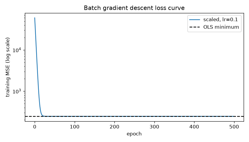
Figure 2. Lab 2 loss curve with standardised features and \(\eta = 0.1\). The dashed line is the closed-form OLS minimum (MSE 245.09).
When to choose which:
| Situation | Use |
|---|---|
| Data fits in memory, \(p\) moderate | Closed form via QR/SVD (lstsq, LinearRegression): exact, no tuning |
| Very large \(n\), data does not fit in memory | Mini-batch GD / SGD (SGDRegressor) |
| Streaming data, online updates | SGD with incremental updates |
| Linear layer inside a larger model trained by gradients | GD, by construction |
10. Regularisation: Ridge, Lasso and Elastic Net#
Regularisation adds a penalty on coefficient size. It accepts a little bias for a potentially large reduction in variance. Two rules always apply: standardise features first (the penalty treats all coefficients alike, and their size depends on units), and do not penalise the intercept (libraries centre the data and fit it separately).
Ridge (L2)#
- \(\lambda \ge 0\) is the penalty strength; \(\lVert \boldsymbol{\beta} \rVert^2\) is the sum of squared non-intercept coefficients. The closed form assumes centred \(\mathbf{X}\) and \(\mathbf{y}\).
- For \(\lambda > 0\), \(\mathbf{X}^\top\mathbf{X} + \lambda\mathbf{I}\) is positive definite, so it is always invertible, even with perfect collinearity or \(p > n\).
- Adding \(\lambda\) to every eigenvalue lowers the condition number from \(\lambda_{\max}/\lambda_{\min}\) to \((\lambda_{\max} + \lambda)/(\lambda_{\min} + \lambda)\).
- In SVD terms, Ridge multiplies each OLS component by \(d_j^2/(d_j^2 + \lambda)\), where \(d_j\) are the singular values of \(\mathbf{X}\). It shrinks most the directions with small \(d_j\): the unstable, collinear ones.
- Coefficients shrink towards 0 but are never exactly 0 for finite \(\lambda\).
- scikit-learn's
Ridge(alpha=α)minimises exactly this objective, soalpha= \(\lambda\).RidgeCVpicksalphaby efficient leave-one-out CV by default, or by k-fold CV if you passcv.
Lasso (L1)#
- \(\alpha\) is the penalty strength in scikit-learn's scaling. Because of the \(1/(2n)\) factor, a Lasso
alphais not comparable with a Ridgealpha. - \(\lVert \boldsymbol{\beta} \rVert_1\) is the L1 norm, the sum of absolute coefficient values.
- There is no closed form in general; scikit-learn uses coordinate descent.
Why Lasso gives exact zeros. With an orthonormal design (\(\mathbf{X}^\top\mathbf{X} = \mathbf{I}\)) and objective \(\tfrac{1}{2}\lVert \mathbf{y} - \mathbf{X}\boldsymbol{\beta} \rVert^2 + \lambda\lVert \boldsymbol{\beta} \rVert_1\), each coefficient is the OLS value \(z_j\) passed through soft-thresholding. Ridge (with penalty \(\tfrac{\lambda}{2}\lVert \boldsymbol{\beta} \rVert^2\)) shrinks proportionally:
- \(z_j\) is the OLS coefficient; \(\operatorname{sign}(z_j)\) is +1 or −1.
- With \(\lambda = 1\): \(z = 3.0\) gives Lasso 2.0 and Ridge 1.5; \(z = 0.5\) gives Lasso 0.0 and Ridge 0.25.
Geometrically, the L1 constraint region \(\lVert \boldsymbol{\beta} \rVert_1 \le t\) is a diamond with corners on the axes, and the elliptical squared-error contours usually touch it at a corner, where some coordinates are 0. The L2 ball has no corners. Lasso caveats: among highly correlated features it picks one somewhat arbitrarily and the choice can change between samples; with \(p > n\) it selects at most \(n\) features; kept coefficients are biased towards 0.
Elastic Net#
- \(\rho\) is scikit-learn's
l1_ratio, between 0 and 1: \(\rho = 1\) is Lasso, \(\rho = 0\) is Ridge. Elastic Net keeps sparsity while sharing weight across correlated features. Tune both \(\alpha\) and \(\rho\) withElasticNetCV.
Choosing the penalty: cross-validate over a log grid (for example \(10^{-3}\) to \(10^{3}\)). Optionally apply the one-standard-error rule: take the largest penalty whose CV error is within one standard error of the best. Do not read p-values from a regularised fit as if it were OLS.
Ridge on collinear data: worked example (c)#
Same 8 synthetic rows as Example (b). Features are standardised (\(\mathbf{Z}\) is the standardised feature matrix), \(y\) is centred, and the closed-form Ridge result is cross-checked against sklearn.linear_model.Ridge:
| \(\lambda\) | \(w_1\) (vCPU) | \(w_2\) (memory) | \(w_3\) (cache) | train \(R^2\) | \(\kappa(\mathbf{Z}^\top\mathbf{Z} + \lambda\mathbf{I})\) | LOOCV RMSE |
|---|---|---|---|---|---|---|
| 0 (OLS) | 2.6955 | 5.9976 | 1.4135 | 0.9996 | 3455.78 | 0.3551 |
| 0.1 | 4.2451 | 4.3932 | 1.3953 | 0.9995 | 154.16 | 0.2908 |
| 1 | 4.0784 | 4.0953 | 1.2364 | 0.9958 | 16.95 | 0.8768 |
| 10 | 2.6610 | 2.6633 | 0.5587 | 0.8451 | 2.60 | 4.7007 |
After the same one-unit change to row 4, OLS moves \((w_1, w_2)\) from (2.70, 6.00) to (7.85, 0.81); Ridge with \(\lambda = 0.1\) moves only from (4.25, 4.39) to (4.46, 4.15). Training \(R^2\) always falls as \(\lambda\) grows; leave-one-out error first improves (\(\lambda = 0.1\)), then worsens as shrinkage becomes too strong (\(\lambda = 10\) underfits).
Caveat: made-up data. Example (c) has 8 synthetic rows. It shows the mechanism (stability, conditioning, bias–variance), not a general claim that \(\lambda = 0.1\) is a good value.
OLS vs Ridge vs Lasso on real data (Lab 3, scikit-learn diabetes)#
The diabetes dataset ships with scikit-learn: 442 patients, 10 baseline features (age, sex, BMI, average blood pressure, six blood serum measurements s1–s6), and a target that measures disease progression one year later. Lab 3 loads it in raw units (scaled=False), holds out 20% (random_state=42), and fits each model inside Pipeline(StandardScaler, model).
| Model | Penalty chosen | Train \(R^2\) | Test \(R^2\) | Test RMSE | Test MAE |
|---|---|---|---|---|---|
| OLS | none | 0.5279 | 0.4526 | 53.85 | 42.79 |
| RidgeCV | alpha = 1.2589 | 0.5275 | 0.4544 | 53.77 | 42.82 |
| LassoCV | alpha = 0.5420 | 0.5244 | 0.4613 | 53.43 | 42.84 |
Coefficients on the standardised scale (target units per one SD of the feature):
| Feature | OLS | Ridge | Lasso |
|---|---|---|---|
| age | 1.75 | 1.82 | 1.29 |
| sex | −11.51 | −11.43 | −10.30 |
| bmi | 25.61 | 25.75 | 26.23 |
| bp | 16.83 | 16.71 | 16.13 |
| s1 | −44.45 | −32.84 | −11.37 |
| s2 | 24.64 | 15.64 | 0.00 |
| s3 | 7.68 | 2.57 | −6.65 |
| s4 | 13.14 | 11.51 | 7.12 |
| s5 | 35.16 | 30.67 | 23.05 |
| s6 | 2.35 | 2.48 | 2.31 |
The serum measures are strongly collinear (VIF: s1 55.25, s2 35.76, s3 14.29, s5 10.07), which is why OLS gives s1 and s2 large opposite-signed coefficients. Ridge shrinks them; Lasso sets s2 exactly to 0 and cuts s1 from −44.45 to −11.37. Note that s3 changes sign under Lasso: with collinear features, individual coefficients are not stable enough to interpret one at a time.
Caveat: do not call Lasso "better" on this evidence. The test RMSE gap between the three models is under 0.5 on a target whose SD is 77.09. That is smaller than split-to-split variation. OLS 5-fold CV \(R^2\) on the training set ranges from 0.411 to 0.537 across folds (mean 0.4804, SD 0.0409), and re-running with
random_state=0drops test \(R^2\) to 0.3322 (OLS), 0.3348 (Ridge) and 0.3354 (Lasso). On this data, regularisation buys stability and a slightly simpler model, not a meaningful accuracy gain. To compare models properly, use repeated CV and look at the spread, not one split.
11. Full runnable code: worked example (a) end to end#
This script reproduces every number in Section 5: the normal equations, lstsq, statsmodels inference, VIF, leverage, Cook's distance and Durbin–Watson. Save it as example_a_multiple_regression.py (it is also in the download zip) and run it inside the virtual environment from the setup step.
"""Worked Example (a): multiple linear regression on 6 rows (synthetic teaching data).
Normal equation from scratch, cross-checked with np.linalg.lstsq and statsmodels,
plus R^2, adjusted R^2, VIF, leverage, Cook's distance and Durbin-Watson."""
import numpy as np
import statsmodels.api as sm
from statsmodels.stats.outliers_influence import variance_inflation_factor
from statsmodels.stats.stattools import durbin_watson

x1 = np.array([1, 2, 3, 4, 5, 6], dtype=float)      # VMs
x2 = np.array([2, 1, 3, 3, 5, 4], dtype=float)      # storage, TB
y  = np.array([5, 7, 12, 13, 19, 19], dtype=float)  # monthly bill, $100s

X = np.column_stack([np.ones_like(x1), x1, x2])     # design matrix with intercept column
n, k = X.shape                                       # k = p + 1 parameters
p = k - 1

XtX, Xty = X.T @ X, X.T @ y
print("X^T X =\n", XtX.astype(int))
print("X^T y =", Xty.astype(int))
print("det(X^T X) = %.1f" % np.linalg.det(XtX))

beta_solve = np.linalg.solve(XtX, Xty)               # normal equations (teaching)
beta_lstsq = np.linalg.lstsq(X, y, rcond=None)[0]    # SVD-based (what you use in practice)
print("beta (solve) =", np.round(beta_solve, 4))
print("beta (lstsq) =", np.round(beta_lstsq, 4))

y_hat = X @ beta_lstsq
e = y - y_hat
ss_res = e @ e
ss_tot = np.sum((y - y.mean()) ** 2)
r2 = 1 - ss_res / ss_tot
adj_r2 = 1 - (1 - r2) * (n - 1) / (n - p - 1)
print("residuals    =", np.round(e, 4), " sum = %.1e" % e.sum())
print("SS_res = %.4f  SS_tot = %.4f" % (ss_res, ss_tot))
print("R^2 = %.4f  adjusted R^2 = %.4f  RMSE = %.4f" % (r2, adj_r2, np.sqrt(ss_res / n)))

fit = sm.OLS(y, X).fit()                              # X already has the constant
print("statsmodels params =", np.round(fit.params, 4))
print("statsmodels SE     =", np.round(fit.bse, 4))
print("statsmodels p      =", np.round(fit.pvalues, 4))
print("statsmodels R^2 = %.4f  adj R^2 = %.4f  F = %.1f" % (fit.rsquared, fit.rsquared_adj, fit.fvalue))

vif = [variance_inflation_factor(X, j) for j in range(1, k)]
infl = fit.get_influence()
print("VIF (x1, x2)       =", np.round(vif, 4))
print("leverage h_ii      =", np.round(infl.hat_matrix_diag, 4), " sum = %.1f" % infl.hat_matrix_diag.sum())
print("Cook's distance    =", np.round(infl.cooks_distance[0], 4))
print("Durbin-Watson      = %.4f" % durbin_watson(e))
print("prediction at x1=4, x2=4:", round(float(np.array([1, 4, 4]) @ beta_lstsq), 4))
python example_a_multiple_regression.pyExpected output (verified):
X^T X =
 [[ 6 21 18]
 [21 91 74]
 [18 74 64]]
X^T y = [ 75 316 263]
det(X^T X) = 324.0
beta (solve) = [0.6667 2.1667 1.4167]
beta (lstsq) = [0.6667 2.1667 1.4167]
residuals    = [-0.6667  0.5833  0.5833 -0.5833  0.4167 -0.3333]  sum = 2.5e-14
SS_res = 1.7500  SS_tot = 171.5000
R^2 = 0.9898  adjusted R^2 = 0.9830  RMSE = 0.5401
statsmodels params = [0.6667 2.1667 1.4167]
statsmodels SE     = [0.7915 0.3287 0.4348]
statsmodels p      = [0.4615 0.0071 0.0472]
statsmodels R^2 = 0.9898  adj R^2 = 0.9830  F = 145.5
VIF (x1, x2)       = [3.2407 3.2407]
leverage h_ii      = [0.6296 0.6574 0.213  0.213  0.6574 0.6296]  sum = 3.0
Cook's distance    = [1.1657 1.0891 0.0669 0.0669 0.5557 0.2914]
Durbin-Watson      = 2.5635
prediction at x1=4, x2=4: 15.0
Reading the output:
beta (solve)andbeta (lstsq)match the hand result \([2/3, 13/6, 17/12]\).R^2 = 0.9898(97/98) andadjusted R^2 = 0.9830(289/294).- The residual sum prints as a tiny number (here
2.5e-14), not exactly 0. That is floating-point round-off; your last digits may differ. - With only two features, both VIFs equal \(1/(1 - 0.8315^2) \approx 3.24\), below the usual screening thresholds.
Durbin-Watson = 2.5635is just above the 1.5–2.5 rule of thumb, and it means nothing here: the six teams have no natural order. This is a case where a rule of thumb should be ignored.
12. Hands-on labs#
All three labs run on your own machine with the setup above: no cloud account, no cost, no network after pip install. Expected outputs were produced by running the scripts. Digits beyond the 4th–6th significant figure and round-off values (\(10^{-13}\) to \(10^{-16}\)) can differ across machines, BLAS libraries and package versions.
Download all lab scripts and expected outputs (zip) linreg-expert-labs.zip · 10 files · 11 KB
Lab 1: normal equation from scratch, cross-checked six ways#
Objective. Implement \(\hat{\boldsymbol{\beta}} = (\mathbf{X}^\top\mathbf{X})^{-1}\mathbf{X}^\top\mathbf{y}\), confirm that six routes give the same coefficients, verify \(\mathbf{X}^\top\mathbf{e} = \mathbf{0}\), \(\operatorname{trace}(\mathbf{H}) = p+1\) and \(\mathbf{H}^2 = \mathbf{H}\), and measure why explicit inversion is avoided.
Requirements. Setup done; Sections 2–3 read. Runs in a few seconds.
Steps.
- Save the script as
lab1_normal_equation.py. - Run
python lab1_normal_equation.py. - Compare with the expected output and the checks below.
"""Lab 1: OLS via the normal equation from scratch, cross-checked with
np.linalg.lstsq, QR, pinv and scikit-learn LinearRegression."""
import numpy as np
from sklearn.linear_model import LinearRegression

rng = np.random.default_rng(42)
n, p = 200, 3
X_raw = rng.normal(size=(n, p))                     # 3 features
beta_true = np.array([4.0, 2.0, -3.0, 0.5])          # [intercept, b1, b2, b3]
X = np.column_stack([np.ones(n), X_raw])             # design matrix with intercept column
y = X @ beta_true + rng.normal(scale=1.0, size=n)    # noise sd = 1

# 1) Normal equation, two ways
XtX, Xty = X.T @ X, X.T @ y
beta_inv   = np.linalg.inv(XtX) @ Xty                # explicit inverse (teaching only)
beta_solve = np.linalg.solve(XtX, Xty)               # solve linear system (better)

# 2) Library / factorisation routes
beta_lstsq, _, rank, sv = np.linalg.lstsq(X, y, rcond=None)   # SVD-based
Q, R = np.linalg.qr(X)
beta_qr   = np.linalg.solve(R, Q.T @ y)              # QR route
beta_pinv = np.linalg.pinv(X) @ y                    # Moore-Penrose pseudo-inverse
sk = LinearRegression().fit(X_raw, y)                # sklearn adds intercept itself
beta_sk = np.r_[sk.intercept_, sk.coef_]

print("true beta      :", beta_true)
for name, b in [("inv", beta_inv), ("solve", beta_solve), ("lstsq", beta_lstsq),
                ("qr", beta_qr), ("pinv", beta_pinv), ("sklearn", beta_sk)]:
    print(f"{name:<15}: {np.round(b, 4)}   max|diff vs lstsq| = {np.max(np.abs(b - beta_lstsq)):.2e}")
print("rank(X) =", rank, " singular values:", np.round(sv, 3))

# 3) Properties of the OLS solution
y_hat = X @ beta_lstsq
e = y - y_hat
H = X @ np.linalg.solve(XtX, X.T)                    # hat matrix
print("sum of residuals          :", f"{e.sum():.2e}")
print("max |X^T e| (orthogonality):", f"{np.max(np.abs(X.T @ e)):.2e}")
print("trace(H) (= p+1)           :", round(np.trace(H), 6))
print("H idempotent (max|HH-H|)   :", f"{np.max(np.abs(H @ H - H)):.2e}")
r2 = 1 - (e @ e) / np.sum((y - y.mean())**2)
print("R^2 (manual) =", round(r2, 4), " R^2 (sklearn) =", round(sk.score(X_raw, y), 4))

# 4) Why not invert X^T X?  Condition number squares.
x1 = rng.normal(size=n)
X_bad = np.column_stack([np.ones(n), x1, x1 + 1e-6 * rng.normal(size=n)])
print("cond(X_bad)       = %.3e" % np.linalg.cond(X_bad))
print("cond(X_bad^T X_bad) = %.3e  (approx. cond(X)^2)" % np.linalg.cond(X_bad.T @ X_bad))
Expected output:
true beta      : [ 4.   2.  -3.   0.5]
inv            : [ 3.9629  2.0368 -3.0076  0.4483]   max|diff vs lstsq| = 2.66e-15
solve          : [ 3.9629  2.0368 -3.0076  0.4483]   max|diff vs lstsq| = 2.22e-15
lstsq          : [ 3.9629  2.0368 -3.0076  0.4483]   max|diff vs lstsq| = 0.00e+00
qr             : [ 3.9629  2.0368 -3.0076  0.4483]   max|diff vs lstsq| = 1.33e-15
pinv           : [ 3.9629  2.0368 -3.0076  0.4483]   max|diff vs lstsq| = 6.66e-15
sklearn        : [ 3.9629  2.0368 -3.0076  0.4483]   max|diff vs lstsq| = 1.78e-15
rank(X) = 4  singular values: [14.665 14.421 13.663 12.599]
sum of residuals          : -3.60e-13
max |X^T e| (orthogonality): 3.64e-13
trace(H) (= p+1)           : 4.0
H idempotent (max|HH-H|)   : 4.16e-17
R^2 (manual) = 0.921  R^2 (sklearn) = 0.921
cond(X_bad)       = 2.089e+06
cond(X_bad^T X_bad) = 4.358e+12  (approx. cond(X)^2)
Checks.
- All six coefficient vectors agree to about \(10^{-14}\) or better. The estimates (3.96, 2.04, −3.01, 0.45) are close to, not equal to, the true values (4, 2, −3, 0.5) because of the noise term.
sum of residualsandmax |X^T e|are zero up to round-off: the normal equations hold.trace(H) = 4.0equals \(p + 1\) (3 features + intercept).- \((2.089 \times 10^6)^2 \approx 4.36 \times 10^{12}\): the condition number squares when you form \(\mathbf{X}^\top\mathbf{X}\).
Extension: an exactly singular design. Append these lines to the script:
X_sing = np.column_stack([np.ones(n), x1, x1])
try:
    print("inv:", np.linalg.inv(X_sing.T @ X_sing) @ X_sing.T @ y)
except np.linalg.LinAlgError as err:
    print("inv failed:", err)
b, _, r, _ = np.linalg.lstsq(X_sing, y, rcond=None)
print("lstsq:", np.round(b, 4), "rank =", r)
Reference output:
inv failed: Singular matrix
lstsq: [4.1809 0.0067 0.0067] rank = 2
np.linalg.lstsq returns the minimum-norm solution, splits the shared coefficient equally between the two identical columns, and reports rank = 2. On other inputs np.linalg.inv can return huge meaningless values without raising an error, which is worse than failing.
Troubleshooting.
| Symptom | Cause and fix |
|---|---|
ModuleNotFoundError: No module named 'sklearn' |
The virtual environment is not active. Run source .venv/bin/activate (PowerShell: .venv\Scripts\Activate.ps1) and re-run. |
The max diff vs lstsq values differ slightly from the reference |
Normal floating-point differences across machines. Anything around \(10^{-13}\) or smaller is agreement. |
| Coefficients differ from 3.9629 etc. in the 2nd decimal | You changed the seed or n. The script uses default_rng(42) and n = 200. |
Cleanup: rm lab1_normal_equation.py
Lab 2: batch gradient descent, feature scaling and the loss curve#
Objective. Implement batch GD for MSE; show that unscaled features force a tiny learning rate or diverge; show that standardised features converge in tens of epochs; map scaled coefficients back and match the closed-form OLS solution.
Requirements. Setup done; Lab 1; Section 9 read. Writes one PNG to the current folder.
Steps.
- Save the script as
lab2_gradient_descent.py. - Run
python lab2_gradient_descent.py. - Open
lab2_loss_curve.pngand confirm the curve reaches the dashed OLS line (compare with Figure 2).
"""Lab 2: Batch gradient descent for multiple linear regression, with and
without feature scaling, compared with the closed-form OLS solution."""
import numpy as np
import matplotlib
matplotlib.use("Agg")                     # no display needed; writes PNG
import matplotlib.pyplot as plt

rng = np.random.default_rng(7)
n = 500
size_sqft = rng.uniform(500, 3500, n)    # large scale feature
rooms     = rng.integers(1, 6, n).astype(float)
age_years = rng.uniform(0, 40, n)
X_raw = np.column_stack([size_sqft, rooms, age_years])
y = 50 + 0.12 * size_sqft + 8.0 * rooms - 1.5 * age_years + rng.normal(0, 15, n)

def mse(X, y, w):                         # X includes the intercept column
    r = X @ w - y
    return (r @ r) / len(y)

def batch_gd(X, y, lr, epochs):
    np.seterr(over="ignore", invalid="ignore")   # divergence is shown on purpose
    w = np.zeros(X.shape[1])
    hist = []
    for _ in range(epochs):
        grad = (2 / len(y)) * X.T @ (X @ w - y)   # gradient of MSE
        w -= lr * grad
        hist.append(mse(X, y, w))
        if not np.isfinite(hist[-1]):
            break
    return w, np.array(hist)

# Closed-form reference on the original scale
X1 = np.column_stack([np.ones(n), X_raw])
w_ols = np.linalg.lstsq(X1, y, rcond=None)[0]
print("OLS (lstsq) original scale :", np.round(w_ols, 4))

# A) Unscaled features
for lr in [1e-7, 1e-6]:
    w_u, h_u = batch_gd(X1, y, lr=lr, epochs=2000)
    print(f"unscaled lr={lr:g}: final MSE={h_u[-1]:.4g}  epochs run={len(h_u)}")

# B) Standardised features (fit mean/std on the data used for training)
mu, sd = X_raw.mean(0), X_raw.std(0)
Xs = np.column_stack([np.ones(n), (X_raw - mu) / sd])
w_s, h_s = batch_gd(Xs, y, lr=0.1, epochs=500)
# Map back to the original scale: b_j = w_j / sd_j ; b0 = w0 - sum(w_j * mu_j / sd_j)
b = w_s[1:] / sd
b0 = w_s[0] - np.sum(w_s[1:] * mu / sd)
w_back = np.r_[b0, b]
print("GD (scaled) mapped back     :", np.round(w_back, 4))
print("max |GD - OLS|              : %.2e" % np.max(np.abs(w_back - w_ols)))
print("final MSE (GD scaled)       : %.4f" % h_s[-1])
print("MSE of OLS                  : %.4f" % mse(X1, y, w_ols))
print("cond(X^T X), unscaled design : %.3e" % np.linalg.cond(X1.T @ X1))
print("cond(X^T X), scaled design   : %.3f" % np.linalg.cond(Xs.T @ Xs))
# GD on MSE is stable only if lr < 1 / lambda_max((1/n) X^T X)
for tag, A in [("unscaled", X1), ("scaled", Xs)]:
    lmax = np.linalg.eigvalsh(A.T @ A / n).max()
    print(f"largest stable lr, {tag:<8}: {1/lmax:.3e}")

# Too large a learning rate on scaled data
_, h_big = batch_gd(Xs, y, lr=1.1, epochs=50)
print("scaled lr=1.1: MSE after %d epochs = %.3e (diverges)" % (len(h_big), h_big[-1]))

plt.figure(figsize=(7, 4))
plt.plot(h_s, label="scaled, lr=0.1")
plt.yscale("log"); plt.xlabel("epoch"); plt.ylabel("training MSE (log scale)")
plt.axhline(mse(X1, y, w_ols), ls="--", c="k", label="OLS minimum")
plt.legend(); plt.title("Batch gradient descent loss curve"); plt.tight_layout()
plt.savefig("lab2_loss_curve.png", dpi=120)
print("saved lab2_loss_curve.png")
Expected output:
OLS (lstsq) original scale : [54.4472  0.1189  7.4043 -1.513 ]
unscaled lr=1e-07: final MSE=1017  epochs run=2000
unscaled lr=1e-06: final MSE=inf  epochs run=160
GD (scaled) mapped back     : [54.4472  0.1189  7.4043 -1.513 ]
max |GD - OLS|              : 7.82e-14
final MSE (GD scaled)       : 245.0873
MSE of OLS                  : 245.0873
cond(X^T X), unscaled design : 6.667e+07
cond(X^T X), scaled design   : 1.056
largest stable lr, unscaled: 2.059e-07
largest stable lr, scaled  : 9.745e-01
scaled lr=1.1: MSE after 50 epochs = 3.573e+13 (diverges)
saved lab2_loss_curve.png
Checks.
GD (scaled) mapped backequalsOLS (lstsq);max |GD - OLS|is far below \(10^{-10}\).lr = 1e-7is below the unscaled limit of 2.06 × 10⁻⁷, so it is stable, but after 2000 epochs MSE is still about 1017 (the minimum is 245.09).lr = 1e-6is above the limit and diverges.- With scaling the limit is about 0.97:
lr = 0.1converges andlr = 1.1diverges.
Troubleshooting.
| Symptom | Cause and fix |
|---|---|
final MSE=inf for lr=1e-06 |
Expected. That run demonstrates divergence; the script suppresses the overflow warnings on purpose. |
| No window opens for the plot | Expected. The script uses the non-interactive Agg backend and writes lab2_loss_curve.png instead. |
| Your own GD never reaches the OLS MSE | Check that you scaled with the training mean and SD, kept the intercept column unscaled, and used the \(2/n\) factor in the gradient. |
Cleanup: rm lab2_gradient_descent.py lab2_loss_curve.png
Lab 3: end-to-end multiple regression on the diabetes dataset#
Objective. Build a leakage-safe pipeline (scaling + model), split train/test, run 5-fold CV, get statsmodels inference, compute VIF, run residual diagnostics (Breusch–Pagan, Jarque–Bera, Shapiro–Wilk, Durbin–Watson, Cook's distance, leverage), compare classical and HC3 standard errors, and compare RidgeCV and LassoCV with OLS on the same split.
Requirements. Setup done; Labs 1–2; Sections 7–10 read. scikit-learn 1.1 or newer (for load_diabetes(scaled=False)). The data ships inside scikit-learn, so nothing is downloaded.
Steps.
- Save the script as
lab3_diabetes_end_to_end.py. - Run
python lab3_diabetes_end_to_end.py. - Read the output section by section with the notes below, and open
lab3_residual_diagnostics.png(compare with Figure 1).
"""Lab 3: End-to-end multiple linear regression on the scikit-learn
diabetes dataset (ships inside scikit-learn; no download needed)."""
import numpy as np, pandas as pd
import matplotlib
matplotlib.use("Agg")
import matplotlib.pyplot as plt
import statsmodels.api as sm
from statsmodels.stats.outliers_influence import variance_inflation_factor
from statsmodels.stats.diagnostic import het_breuschpagan
from statsmodels.stats.stattools import durbin_watson, jarque_bera
from scipy import stats
from sklearn.datasets import load_diabetes
from sklearn.model_selection import train_test_split, KFold, cross_val_score
from sklearn.pipeline import Pipeline
from sklearn.preprocessing import StandardScaler
from sklearn.linear_model import LinearRegression, RidgeCV, LassoCV
from sklearn.metrics import r2_score, mean_squared_error, mean_absolute_error

pd.set_option("display.width", 120)
# ---- 1. Load raw (unscaled) features so that our own scaler matters --------
data = load_diabetes(as_frame=True, scaled=False)
X, y = data.data, data.target
print("Step 1 | shape:", X.shape, "| target mean = %.2f, sd = %.2f" % (y.mean(), y.std()))

# ---- 2. Hold out a test set BEFORE any fitting (prevents leakage) ----------
X_tr, X_te, y_tr, y_te = train_test_split(X, y, test_size=0.2, random_state=42)
print("Step 2 | train:", X_tr.shape, " test:", X_te.shape)

# ---- 3. Pipeline + 5-fold CV on the training set only ----------------------
kf = KFold(n_splits=5, shuffle=True, random_state=42)
ols_pipe = Pipeline([("scale", StandardScaler()), ("model", LinearRegression())])
cv_r2 = cross_val_score(ols_pipe, X_tr, y_tr, cv=kf, scoring="r2")
cv_rmse = -cross_val_score(ols_pipe, X_tr, y_tr, cv=kf, scoring="neg_root_mean_squared_error")
print("Step 3 | OLS 5-fold CV R2  : mean %.4f  sd %.4f  folds %s" % (cv_r2.mean(), cv_r2.std(), np.round(cv_r2, 3)))
print("       | OLS 5-fold CV RMSE: mean %.2f" % cv_rmse.mean())

def evaluate(name, pipe):
    pipe.fit(X_tr, y_tr)
    pred = pipe.predict(X_te)
    return dict(model=name,
                train_R2=r2_score(y_tr, pipe.predict(X_tr)),
                test_R2=r2_score(y_te, pred),
                test_RMSE=np.sqrt(mean_squared_error(y_te, pred)),
                test_MAE=mean_absolute_error(y_te, pred))

rows = [evaluate("OLS", ols_pipe)]
print("Step 3 | OLS test R2 = %.4f, RMSE = %.2f" % (rows[0]["test_R2"], rows[0]["test_RMSE"]))

# ---- 4. statsmodels OLS for inference (training data, original units) ------
Xc_tr = sm.add_constant(X_tr)
sm_fit = sm.OLS(y_tr, Xc_tr).fit()
print("\nStep 4 | statsmodels OLS summary (training set)")
print(sm_fit.summary())

# ---- 5. VIF (training features, with constant in the design) ---------------
vif = pd.Series([variance_inflation_factor(Xc_tr.values, i) for i in range(1, Xc_tr.shape[1])],
                index=X_tr.columns, name="VIF").round(2)
print("\nStep 5 | VIF per feature\n", vif.sort_values(ascending=False).to_string())

# ---- 6. Residual diagnostics ----------------------------------------------
resid, fitted = sm_fit.resid, sm_fit.fittedvalues
bp_lm, bp_p, _, _ = het_breuschpagan(resid, Xc_tr)
jb, jb_p, skew, kurt = jarque_bera(resid)
sh_w, sh_p = stats.shapiro(resid)
dw = durbin_watson(resid)
infl = sm_fit.get_influence()
cooks = infl.cooks_distance[0]
lev = infl.hat_matrix_diag
n_tr, k = Xc_tr.shape
print("\nStep 6 | Breusch-Pagan LM = %.3f, p = %.4f" % (bp_lm, bp_p))
print("       | Jarque-Bera = %.3f, p = %.4f (skew %.3f, kurtosis %.3f)" % (jb, jb_p, skew, kurt))
print("       | Shapiro-Wilk W = %.4f, p = %.4f" % (sh_w, sh_p))
print("       | Durbin-Watson = %.3f" % dw)
print("       | points with Cook's D > 4/n (%.4f): %d ; max Cook's D = %.4f" % (4 / n_tr, (cooks > 4 / n_tr).sum(), cooks.max()))
print("       | points with leverage > 2k/n (%.4f): %d" % (2 * k / n_tr, (lev > 2 * k / n_tr).sum()))
print("       | statsmodels condition number (unscaled design) = %.1f" % sm_fit.condition_number)

# Heteroscedasticity-robust (HC3) standard errors: same coefficients, different SEs
hc3 = sm.OLS(y_tr, Xc_tr).fit(cov_type="HC3")
cmp = pd.DataFrame({"coef_OLS": sm_fit.params, "coef_HC3": hc3.params,
                    "SE_classic": sm_fit.bse, "SE_HC3": hc3.bse,
                    "p_classic": sm_fit.pvalues, "p_HC3": hc3.pvalues}).round(4)
print("       | classic vs HC3 robust inference (coefficients identical, SEs differ)")
print(cmp.to_string())

fig, ax = plt.subplots(1, 2, figsize=(11, 4.2))
ax[0].scatter(fitted, resid, s=12, alpha=.6); ax[0].axhline(0, c="k", lw=1)
ax[0].set_xlabel("fitted value"); ax[0].set_ylabel("residual"); ax[0].set_title("Residuals vs fitted")
sm.qqplot(resid, line="45", fit=True, ax=ax[1]); ax[1].set_title("Normal Q-Q of residuals")
plt.tight_layout(); plt.savefig("lab3_residual_diagnostics.png", dpi=120)
print("       | saved lab3_residual_diagnostics.png")

# ---- 7. Regularised models: RidgeCV and LassoCV inside pipelines -----------
ridge_pipe = Pipeline([("scale", StandardScaler()),
                       ("model", RidgeCV(alphas=np.logspace(-3, 3, 61)))])
lasso_pipe = Pipeline([("scale", StandardScaler()),
                       ("model", LassoCV(cv=kf, random_state=42, max_iter=50000))])
rows.append(evaluate("RidgeCV", ridge_pipe))
rows.append(evaluate("LassoCV", lasso_pipe))
print("\nStep 7 | RidgeCV alpha = %.4f" % ridge_pipe.named_steps["model"].alpha_)
print("       | LassoCV alpha = %.4f" % lasso_pipe.named_steps["model"].alpha_)

coefs = pd.DataFrame({
    "OLS": ols_pipe.named_steps["model"].coef_,
    "Ridge": ridge_pipe.named_steps["model"].coef_,
    "Lasso": lasso_pipe.named_steps["model"].coef_}, index=X.columns).round(2)
print("       | coefficients on the standardised scale (target units per 1 SD of feature)")
print(coefs.to_string())
print("       | Lasso zero coefficients:", list(coefs.index[coefs["Lasso"] == 0]))

print("\nStep 8 | Test-set comparison (same split, random_state=42)")
print(pd.DataFrame(rows).set_index("model").round(4).to_string())
Expected output (the statsmodels Date and Time lines will show your own run time):
Step 1 | shape: (442, 10) | target mean = 152.13, sd = 77.09
Step 2 | train: (353, 10)  test: (89, 10)
Step 3 | OLS 5-fold CV R2  : mean 0.4804  sd 0.0409  folds [0.47  0.537 0.411 0.491 0.493]
       | OLS 5-fold CV RMSE: mean 55.39
Step 3 | OLS test R2 = 0.4526, RMSE = 53.85

Step 4 | statsmodels OLS summary (training set)
                            OLS Regression Results
==============================================================================
Dep. Variable:                 target   R-squared:                       0.528
Model:                            OLS   Adj. R-squared:                  0.514
Method:                 Least Squares   F-statistic:                     38.25
Date:                Fri, 02 Oct 2026   Prob (F-statistic):           5.41e-50
Time:                        04:48:13   Log-Likelihood:                -1906.1
No. Observations:                 353   AIC:                             3834.
Df Residuals:                     342   BIC:                             3877.
Df Model:                          10
Covariance Type:            nonrobust
==============================================================================
                 coef    std err          t      P>|t|      [0.025      0.975]
------------------------------------------------------------------------------
const       -341.3782     74.073     -4.609      0.000    -487.074    -195.683
age            0.1377      0.251      0.549      0.583      -0.356       0.631
sex          -23.0645      6.536     -3.529      0.000     -35.921     -10.208
bmi            5.8464      0.829      7.049      0.000       4.215       7.478
bp             1.1971      0.246      4.873      0.000       0.714       1.680
s1            -1.2817      0.621     -2.065      0.040      -2.503      -0.061
s2             0.8112      0.570      1.423      0.156      -0.310       1.933
s3             0.6017      0.858      0.701      0.484      -1.086       2.289
s4            10.1595      6.841      1.485      0.138      -3.297      23.616
s5            67.1090     17.542      3.826      0.000      32.606     101.612
s6             0.2016      0.304      0.663      0.508      -0.397       0.800
==============================================================================
Omnibus:                        1.457   Durbin-Watson:                   1.794
Prob(Omnibus):                  0.483   Jarque-Bera (JB):                1.412
Skew:                           0.064   Prob(JB):                        0.494
Kurtosis:                       2.718   Cond. No.                     7.07e+03
==============================================================================

Notes:
[1] Standard Errors assume that the covariance matrix of the errors is correctly specified.
[2] The condition number is large, 7.07e+03. This might indicate that there are
strong multicollinearity or other numerical problems.

Step 5 | VIF per feature
 s1     55.25
s2     35.76
s3     14.29
s5     10.07
s4      9.33
bmi     1.57
s6      1.50
bp      1.42
sex     1.27
age     1.22

Step 6 | Breusch-Pagan LM = 19.484, p = 0.0345
       | Jarque-Bera = 1.412, p = 0.4937 (skew 0.064, kurtosis 2.718)
       | Shapiro-Wilk W = 0.9965, p = 0.6398
       | Durbin-Watson = 1.794
       | points with Cook's D > 4/n (0.0113): 18 ; max Cook's D = 0.0277
       | points with leverage > 2k/n (0.0623): 22
       | statsmodels condition number (unscaled design) = 7065.5
       | classic vs HC3 robust inference (coefficients identical, SEs differ)
       coef_OLS  coef_HC3  SE_classic   SE_HC3  p_classic   p_HC3
const -341.3782 -341.3782     74.0728  74.2562     0.0000  0.0000
age      0.1377    0.1377      0.2508   0.2485     0.5834  0.5795
sex    -23.0645  -23.0645      6.5362   6.3047     0.0005  0.0003
bmi      5.8464    5.8464      0.8294   0.8732     0.0000  0.0000
bp       1.1971    1.1971      0.2457   0.2556     0.0000  0.0000
s1      -1.2817   -1.2817      0.6207   0.5944     0.0397  0.0311
s2       0.8112    0.8112      0.5701   0.5336     0.1557  0.1285
s3       0.6017    0.6017      0.8579   0.8345     0.4836  0.4709
s4      10.1595   10.1595      6.8415   6.9594     0.1385  0.1443
s5      67.1090   67.1090     17.5418  16.9635     0.0002  0.0001
s6       0.2016    0.2016      0.3042   0.2916     0.5079  0.4893
       | saved lab3_residual_diagnostics.png

Step 7 | RidgeCV alpha = 1.2589
       | LassoCV alpha = 0.5420
       | coefficients on the standardised scale (target units per 1 SD of feature)
       OLS  Ridge  Lasso
age   1.75   1.82   1.29
sex -11.51 -11.43 -10.30
bmi  25.61  25.75  26.23
bp   16.83  16.71  16.13
s1  -44.45 -32.84 -11.37
s2   24.64  15.64   0.00
s3    7.68   2.57  -6.65
s4   13.14  11.51   7.12
s5   35.16  30.67  23.05
s6    2.35   2.48   2.31
       | Lasso zero coefficients: ['s2']

Step 8 | Test-set comparison (same split, random_state=42)
         train_R2  test_R2  test_RMSE  test_MAE
model
OLS        0.5279   0.4526    53.8534   42.7941
RidgeCV    0.5275   0.4544    53.7650   42.8152
LassoCV    0.5244   0.4613    53.4261   42.8364
Reading the results.
- Generalisation: CV \(R^2\) 0.4804 (folds 0.411–0.537); test \(R^2\) 0.4526, RMSE 53.85. Train \(R^2\) (0.5279) is only modestly above test, so the model is limited by what 10 features can explain (bias), not by overfitting.
- Inference (Step 4):
bmi,bp,s5andsexhave p < 0.001;s1has p ≈ 0.040;age,s2,s3,s4,s6are not individually significant. Adjusted \(R^2\) 0.514 sits below \(R^2\) 0.528 because of the 10-feature penalty. - VIF (Step 5):
s1,s2,s3ands5exceed 10 ands4(9.33) exceeds 5. These serum measures are algebraically related, so their individual coefficients and signs are unstable. - Diagnostics (Step 6): Breusch–Pagan p ≈ 0.0345 (some evidence of non-constant variance); HC3 keeps coefficients identical and shifts SEs without changing significance at 0.05. Normality tests show no evidence against normal residuals. DW is 1.794 on arbitrarily ordered patients. Max Cook's D is 0.0277.
- Regularisation (Steps 7–8): see the comparison table and caveat in Section 10.
Checks.
- The test table has three rows: OLS 0.4526, RidgeCV 0.4544, LassoCV 0.4613.
coef_OLSandcoef_HC3are identical; only SEs and p-values differ.- Split variance: change
random_state=42torandom_state=0in thetrain_test_splitcall only. Reference result: test \(R^2\) 0.3322 (OLS), 0.3348 (Ridge), 0.3354 (Lasso). The Step 8 header still printsrandom_state=42because it is a fixed string. - Leakage experiment: move
StandardScaleroutside the pipeline and fit it on all ofXbefore CV. Plain OLS scores do not change (OLS is scale-equivariant), but for RidgeCV and LassoCV the penalty would be tuned on statistics that include held-out rows. Keep scaling inside the pipeline.
Troubleshooting.
| Symptom | Cause and fix |
|---|---|
TypeError mentioning the keyword scaled |
scikit-learn is older than 1.1. Run pip install --upgrade scikit-learn. |
| Coefficients in Step 4 are very different and the features look already centred | You loaded the default scaled=True version. OLS \(R^2\) is the same; coefficient values differ. Use scaled=False as in the script. |
ConvergenceWarning from LassoCV |
The script sets max_iter=50000. If you change the data or the grid and see it, raise max_iter further. |
| Numbers differ in the 4th decimal or later | Library or BLAS differences. The ranking and the conclusions should not change. |
Cleanup: rm lab3_diabetes_end_to_end.py lab3_residual_diagnostics.png
Full cleanup (all labs):
deactivate
cd ~ && rm -rf ~/lr-expert-labs
Nothing is created outside ~/lr-expert-labs, and no cloud resources are used.
13. Common mistakes#
- Choosing models by training \(R^2\). It never decreases as features are added. Compare by cross-validated error, or at least adjusted \(R^2\), AIC or BIC for in-sample comparisons.
- Forgetting the intercept in statsmodels.
sm.OLS(y, X)does not add a constant. Withoutsm.add_constant(X)the plane is forced through the origin and the reported \(R^2\) is uncentred and not comparable. - The dummy variable trap. All \(k\) levels plus an intercept make \(\mathbf{X}^\top\mathbf{X}\) singular. Use \(k - 1\) dummies for OLS with inference.
- Misreading coefficients. A coefficient is a partial association holding the other included features fixed. It changes when features are added or removed, it is causal only under extra assumptions, and it carries units.
- Thinking heteroscedasticity biases coefficients. It does not (if exogeneity holds); it breaks the classical standard errors. Fix inference with robust SEs; do not drop features because of it.
- Treating VIF cut-offs as laws. VIF > 5 or > 10 are screening conventions. High VIF matters when you need individual coefficients, much less for prediction if the collinearity pattern is stable.
- Leakage through preprocessing. Fitting scalers, imputers, encoders or feature selection on all the data before splitting or CV. Put every data-dependent step inside a
Pipeline. - Regularising unscaled features. Penalties depend on units; without standardisation, features with large numeric ranges are effectively penalised less.
- Random splits on time series or grouped data. Use
TimeSeriesSplitorGroupKFold, otherwise validation is optimistic. Relatedly, p-values reported after stepwise or Lasso selection are over-optimistic. - Extrapolating. Linear models predict outside the training range without complaint. Validate input ranges at serving time.
14. Real-world applications#
These are sensible shapes for multiple regression when relationships are roughly linear and you have numeric history. They are teaching scenarios, not client case studies.
| Use case | Target \(y\) | Features | What to watch |
|---|---|---|---|
| Cloud cost attribution | Monthly bill per team or account | VM count or vCPU-hours, storage TB, data egress GB | Tiered and committed-use pricing break linearity; usage drivers are correlated (check VIF) |
| Capacity planning | p95 latency (ms) | Concurrent requests, payload size, cache hit rate | Latency often curves near saturation; residuals vs load will show it |
| Database query runtime | Query time | Rows scanned, number of joins, index used (dummy) | Often heteroscedastic (big queries vary more): try a log of \(y\) or HC3 SEs |
| Storage and log growth | GB per day | Active users, services deployed, retention days | Time-ordered: check Durbin–Watson and use time-aware splits |
| Support or incident load | Tickets per week | Active tenants, deployments per week | Counts near zero may need a count model instead |
Production concerns#
- Deploy the pipeline, not the coefficients. Serialise the whole fitted
Pipeline(imputation, encoding, scaling, model) so training and serving apply identical transformations. Pin library versions; pickled scikit-learn objects are not guaranteed to load across versions. - Validate inputs. Enforce column names, types, ranges and allowed categories. Out-of-range inputs give confident but unsupported predictions.
- Avoid training–serving skew. Compute features with the same code (or a feature store) offline and online.
- Monitor drift. Data drift (the distribution of \(\mathbf{X}\) moves), concept drift (the relationship changes), label drift. Track feature distributions (for example the population stability index or Kolmogorov–Smirnov tests), prediction distributions and, once labels arrive, rolling RMSE/MAE and residual bias by segment.
- Retrain deliberately. On a schedule, or when drift or error thresholds are crossed. Validate the challenger against the current model on recent data, deploy gradually (shadow or canary), keep rollback.
- Explain and quantify uncertainty. Each prediction decomposes as \(\hat{y} = \beta_0 + \sum_j \beta_j x_j\). Serve prediction intervals where decisions depend on risk and check their coverage. With correlated features, per-feature contributions are not uniquely attributable.
15. Interview questions#
1. Derive the OLS estimator in matrix form. When does it fail to exist?
Minimise \(S(\boldsymbol{\beta}) = \lVert \mathbf{y} - \mathbf{X}\boldsymbol{\beta} \rVert^2\). The gradient \(-2\mathbf{X}^\top\mathbf{y} + 2\mathbf{X}^\top\mathbf{X}\boldsymbol{\beta}\) is zero at \(\mathbf{X}^\top\mathbf{X}\hat{\boldsymbol{\beta}} = \mathbf{X}^\top\mathbf{y}\); the Hessian \(2\mathbf{X}^\top\mathbf{X}\) is positive semi-definite, so it is a minimum. With full column rank the solution \((\mathbf{X}^\top\mathbf{X})^{-1}\mathbf{X}^\top\mathbf{y}\) is unique. It is not unique with linearly dependent columns or \(p + 1 > n\); then drop redundant columns, use the pseudo-inverse, or use Ridge.
2. Why don't libraries compute \((\mathbf{X}^\top\mathbf{X})^{-1}\) directly?
Forming \(\mathbf{X}^\top\mathbf{X}\) squares the condition number, so precision is lost before inversion starts, and inverting is slower and less stable than solving. QR works at the conditioning of \(\mathbf{X}\); SVD also handles rank deficiency. np.linalg.lstsq is SVD-based, and scikit-learn's LinearRegression calls SciPy's lstsq.
3. Explain the hat matrix and leverage.
\(\mathbf{H} = \mathbf{X}(\mathbf{X}^\top\mathbf{X})^{-1}\mathbf{X}^\top\) projects \(\mathbf{y}\) onto the column space: \(\hat{\mathbf{y}} = \mathbf{H}\mathbf{y}\). It is symmetric and idempotent with trace \(p + 1\). The diagonal \(h_{ii}\) is the leverage of row \(i\). Residual variance is \(\sigma^2(1 - h_{ii})\), so high-leverage rows have smaller raw residuals, which is why studentised residuals are used.
4. State the Gauss–Markov assumptions. Where does normality come in?
Linearity in parameters, full column rank, \(\mathbb{E}[\boldsymbol{\varepsilon} \mid \mathbf{X}] = \mathbf{0}\), and \(\operatorname{Var}(\boldsymbol{\varepsilon} \mid \mathbf{X}) = \sigma^2\mathbf{I}\). The first three give unbiasedness; the fourth makes OLS BLUE. Normality is not part of the theorem; it makes t and F exact in small samples.
5. What does heteroscedasticity do to OLS?
Coefficients stay unbiased; OLS loses efficiency and the classical variance formula is wrong, so t-tests and intervals are unreliable. Detect it with residual plots and Breusch–Pagan or White tests; handle it with HC standard errors, a transform of \(y\), or weighted least squares.
6. What is multicollinearity and when does it matter?
Strong linear dependence among features. It inflates \(\operatorname{Var}(\hat{\beta}_j)\) by \(\mathrm{VIF}_j\), destabilises coefficients and weakens individual t-tests while overall fit stays strong. It matters for interpreting coefficients, much less for prediction if the pattern is stable. Remedies: drop or combine features, centre before interactions, Ridge, PCA or PLS.
7. Ridge vs Lasso vs Elastic Net: how do you choose?
Ridge shrinks smoothly, shares weight among correlated features and always has a unique solution, but never produces zeros. Lasso zeros coefficients via soft-thresholding but picks arbitrarily among correlated features. Elastic Net mixes both. Choose by goal (sparsity vs pure prediction) and by cross-validated error, after standardising.
8. Why is polynomial regression still linear regression?
Linearity refers to the parameters: \(\beta_0 + \beta_1 x + \beta_2 x^2\) is a linear combination of the columns \(1, x, x^2\), so OLS and its inference apply unchanged. Powers are collinear, and high degrees extrapolate badly.
9. How do you avoid data leakage in a regression workflow?
Split first; learn every data-dependent transformation inside a Pipeline so it is fitted only on training folds; use TimeSeriesSplit for temporal data and GroupKFold for repeated entities; exclude features unavailable at prediction time; use the test set once.
10. A regression model is in production. What do you monitor, and when do you retrain?
Input schema, missing and out-of-range rates, feature drift; the prediction distribution; rolling RMSE/MAE and residual bias by segment once labels arrive; interval coverage; latency and errors. Retrain on a schedule or on a threshold breach, validate challenger against champion on recent data, deploy gradually, keep rollback, and version the pipeline, data snapshot and libraries.
16. MCQs (10)#
Original teaching questions for this course, not taken from any real exam. Answers follow the questions.
Interactive version: these 10 questions with scoring and instant feedback, plus notes, definitions, worked examples and labs.
Take the interactive quizQ1. Two OLS models are fit on the same \(n = 50\) rows. Model A has 4 features and \(R^2 = 0.800\). Model B adds 4 more (8 in total) and has \(R^2 = 0.810\). Which statement is correct?
A) Model B is better because its \(R^2\) is higher.
B) Adjusted \(R^2\) is about 0.782 for A and about 0.773 for B, so the 4 extra features do not justify the degrees of freedom they use.
C) Adjusted \(R^2\) must be higher for B, because it always moves with \(R^2\).
D) Both have the same adjusted \(R^2\), because it depends only on \(n\).
Q2. A feature \(x_3\) has \(\mathrm{VIF}_3 = 10\). What does this tell you?
A) \(\hat{\beta}_3\) is biased by a factor of 10, so \(x_3\) must be removed.
B) \(x_3\) explains 10% of the variance of \(y\).
C) Regressing \(x_3\) on the other features gives \(R^2 = 0.9\), so the standard error of \(\hat{\beta}_3\) is about \(\sqrt{10} \approx 3.16\) times what it would be if \(x_3\) were uncorrelated with them.
D) The condition number of \(\mathbf{X}\) is exactly 10.
Q3. A model with an intercept one-hot encodes all 4 levels of region (east, north, south, west) and fits plain OLS in statsmodels. What happens, and what is the fix?
A) The 4 dummies sum to the intercept column, so \(\mathbf{X}\) is rank-deficient and \(\mathbf{X}^\top\mathbf{X}\) singular; drop one dummy (the reference level) or drop the intercept.
B) Nothing goes wrong; each dummy coefficient is the difference from the overall mean of \(y\).
C) The dummies must be standardised first, otherwise \(\mathbf{X}^\top\mathbf{X}\) becomes singular.
D) Replace the dummies with one column coded 1, 2, 3, 4.
Q4. You have 200 standardised features and expect about 10 to matter. You want irrelevant coefficients set to exactly zero. Which method, and why?
A) Ridge, because the L2 penalty zeros small coefficients once \(\lambda\) is large enough.
B) Ridge, because the L2 constraint region has corners on the axes.
C) Plain OLS, then remove every feature with p > 0.05; the remaining p-values stay valid.
D) Lasso, because the L1 penalty is not differentiable at 0; its solution soft-thresholds coefficients, so small ones become exactly 0.
Q5. In a large sample, Breusch–Pagan gives p = 0.001 and residuals-vs-fitted shows a funnel. Assuming the other Gauss–Markov assumptions hold, which is correct?
A) The coefficients are now biased and must be re-estimated before interpretation.
B) The coefficients remain unbiased, but classical standard errors, t-tests and intervals are unreliable; robust (for example HC3) standard errors are a standard fix.
C) OLS is still BLUE and classical SEs remain valid because \(n\) is large.
D) \(R^2\) is no longer defined, so fit must be judged by the Breusch–Pagan statistic.
Q6. A house-price model gives price = 40 + 0.15·size_sqft − 12·bedrooms (price in $1000s). On its own, bedrooms correlates positively with price. What does −12 mean?
A) Adding a bedroom to any house will cause its price to fall by $12,000.
B) The model must be wrong, because the sign disagrees with the simple correlation.
C) Comparing houses of the same size, one more bedroom is associated with a predicted price about $12,000 lower, for example because the same floor area is split into smaller rooms.
D) Bedrooms explains −12% of the variance in price.
Q7. Which is NOT required for the Gauss–Markov conclusion that OLS is BLUE?
A) Normally distributed errors.
B) \(\mathbb{E}[\boldsymbol{\varepsilon} \mid \mathbf{X}] = \mathbf{0}\) (strict exogeneity).
C) \(\operatorname{Var}(\boldsymbol{\varepsilon} \mid \mathbf{X}) = \sigma^2\mathbf{I}\).
D) Full column rank of \(\mathbf{X}\).
Q8. With \(n = 40\) rows and \(p = 3\) features plus an intercept, one row has leverage 0.45, an internally studentised residual of 0.1, and Cook's distance about 0.002. What is the best reading?
A) Delete it: its leverage exceeds the \(2(p+1)/n = 0.2\) rule of thumb, so it is distorting the fit.
B) It is a large outlier in \(y\), because high leverage implies a large residual.
C) Its Cook's distance is small because its leverage is small.
D) It has high leverage (unusual feature values) but lies close to the fitted plane, so it has little influence; removing it would barely change the coefficients.
Q9. An engineer standardises the whole dataset with StandardScaler, then runs 5-fold CV of LassoCV on the scaled data and reports the CV score. What is the problem?
A) None; scaling is a linear transformation, so it cannot affect any model's results.
B) The scaler's mean and SD were computed using rows that later serve as validation folds, which leaks information; put the scaler inside a Pipeline so it is re-fit on each training fold.
C) The test folds should be scaled with their own mean and SD.
D) Leakage only matters for tree-based models.
Q10. You have 500 features and 120 rows (\(p > n\)). What is true?
A) OLS has a unique solution; it is just slow, so gradient descent is preferred.
B) Removing the intercept column makes \(\mathbf{X}^\top\mathbf{X}\) invertible.
C) \(\operatorname{rank}(\mathbf{X}) \le 120 < 501\) columns, so \(\mathbf{X}^\top\mathbf{X}\) is singular and infinitely many coefficient vectors reach the same minimum; Ridge with \(\lambda > 0\) makes \(\mathbf{X}^\top\mathbf{X} + \lambda\mathbf{I}\) invertible and gives a unique solution.
D) Gradient descent from any start converges to the same unique OLS coefficients, so rank does not matter.
Answer key#
| Q | Answer | Why |
|---|---|---|
| 1 | B | \(1 - 0.2 \cdot 49/45 \approx 0.7822\) vs \(1 - 0.19 \cdot 49/41 \approx 0.7729\): the penalty for 4 more features outweighs a 0.01 gain in \(R^2\). |
| 2 | C | \(1/(1 - R^2_3) = 10\) gives \(R^2_3 = 0.9\); the SE scales by \(\sqrt{\mathrm{VIF}}\). Collinearity inflates variance; it does not bias. |
| 3 | A | The dummies sum to 1 in every row, which equals the intercept column. Use \(k - 1\) dummies; coefficients become differences from the reference level. |
| 4 | D | Under orthonormal design Lasso gives \(\operatorname{sign}(z)\max(\lvert z \rvert - \lambda, 0)\) and Ridge \(z/(1+\lambda)\), never exactly 0. Selecting by p-value and reporting the same p-values overstates significance. |
| 5 | B | Unbiasedness needs only GM1–GM3. Heteroscedasticity breaks \(\sigma^2(\mathbf{X}^\top\mathbf{X})^{-1}\) and efficiency; a large \(n\) does not repair the classical formula. |
| 6 | C | A partial effect with size held fixed. Sign differences from simple correlations are normal when features are correlated. Reading it causally (A) ignores the "same size" condition. |
| 7 | A | Normality gives exact small-sample t and F distributions; it is not a Gauss–Markov assumption. |
| 8 | D | \(D = (0.1^2/4)\cdot(0.45/0.55) \approx 0.002\). Influence needs leverage and a sizeable residual. Rules of thumb flag rows for inspection, not deletion. |
| 9 | B | Every data-dependent preprocessing step must be learned on training folds only, and Lasso is not scale-invariant. |
| 10 | C | A 120 × 501 matrix has rank at most 120; adding \(\lambda\mathbf{I}\) makes every eigenvalue positive. Gradient descent reaches some minimiser, depending on the start (from zero, the minimum-norm one). |
17. Practice exercises and mini project#
E1. Extrapolation. Using Example (a), predict the bill at \(x_1 = 7\), \(x_2 = 5\). Why should you be cautious?
(Answer: \(\hat{y} = 2/3 + 7 \cdot 13/6 + 5 \cdot 17/12 \approx 22.9167\), about $2,292. \(x_1 = 7\) is outside the observed range of 1 to 6, so this is extrapolation, and with 3 residual degrees of freedom any interval around it is wide.)
E2. Omitted feature. Refit Example (a) with \(x_1\) only. Report the slope, intercept, \(R^2\) and adjusted \(R^2\), and explain why the slope differs from 2.1667.
(Answer: slope 3.0571, intercept 1.8, \(R^2 = 0.9537\), adjusted 0.9421. \(x_1\) and \(x_2\) are correlated (0.8315), so without \(x_2\) the VM slope absorbs part of the storage effect. Adjusted \(R^2\) is lower than the two-feature 0.9830, so \(x_2\) earns its place in-sample.)
E3. VIF by hand. With two features, \(R^2_1\) is the squared correlation between them. Compute VIF for Example (a).
(Answer: \(1/(1 - 0.8315^2) \approx 3.24\); statsmodels prints 3.2407.)
E4. Soft-thresholding. With \(\lambda = 1\) and an orthonormal design, what are the Lasso and Ridge coefficients for an OLS coefficient \(z = -2.0\)? Then for \(z = 0.5\)?
(Answer: for \(z = -2.0\), Lasso \(\operatorname{sign}(-2)\cdot\max(2 - 1, 0) = -1.0\) and Ridge \(-2/(1+1) = -1.0\), equal by coincidence. For \(z = 0.5\), Lasso 0 and Ridge 0.25.)
E5. Split variance. In Lab 3, change only the train_test_split seed to random_state=0. Record test \(R^2\) for the three models and write two sentences on what this means for model comparison.
(Reference: 0.3322 / 0.3348 / 0.3354. One change of split moves \(R^2\) by more than 0.1, while the gap between models stays under 0.01.)
E6. Leakage. In Lab 3, fit StandardScaler on all of X outside the pipeline, then rerun CV for OLS and for LassoCV. Which score is unchanged, and why is the approach still wrong?
(Expected: OLS CV scores are unchanged because OLS is scale-equivariant. For LassoCV, the penalty is tuned on statistics that include validation rows. Run it to see the size of the effect on your machine; do not assume a number.)
E7. Diagnostics write-up. For Lab 3, write a five-line diagnostic summary a reviewer could act on: residual pattern, heteroscedasticity, normality, collinearity, influence. Use only numbers the script prints.
Mini project: explainable price model with honest uncertainty#
Dataset: California housing (sklearn.datasets.fetch_california_housing): 20,640 rows, 8 numeric features (MedInc, HouseAge, AveRooms, AveBedrms, Population, AveOccup, Latitude, Longitude), target MedHouseVal in units of $100,000. It downloads once on first use and is then cached under ~/scikit_learn_data. The target appears capped at about 5.0. Without network access, use the diabetes data from Lab 3.
Deliverables:
- A reproducible script or notebook with fixed seeds and a pinned
requirements.txt. - EDA: distributions, correlation matrix, VIF table, and a justified decision on the capped target rows.
- Baseline
Pipeline(StandardScaler, LinearRegression)with 5-fold CV (mean ± SD of RMSE and \(R^2\)) and one held-out test evaluation. - At least two feature-engineering iterations (for example log of skewed features,
AveBedrms/AveRooms,PolynomialFeatures, spatial bins of latitude/longitude), each backed by CV evidence. - RidgeCV, LassoCV and ElasticNetCV inside pipelines, with a standardised coefficient table.
- statsmodels OLS of the final feature set: summary, Breusch–Pagan, Q-Q plot, Cook's distance, classical vs HC3 SEs.
- Prediction intervals for 5 example rows and an empirical coverage check of 95% intervals on the test set.
- A one-page model card: intended use, data, metrics, limitations (capping, spatial correlation, extrapolation), monitoring plan and retraining trigger.
Suggested rubric: leakage-free evaluation 30% · diagnostics and correct interpretation 25% · regularisation and feature engineering with CV evidence 20% · production readiness (pipeline serialisation, input validation, monitoring plan) 15% · model card clarity 10%.
18. Summary#
- Multiple regression is \(\mathbf{y} = \mathbf{X}\boldsymbol{\beta} + \boldsymbol{\varepsilon}\). OLS minimises \(\lVert \mathbf{y} - \mathbf{X}\boldsymbol{\beta} \rVert^2\), which gives the normal equations \(\mathbf{X}^\top\mathbf{X}\hat{\boldsymbol{\beta}} = \mathbf{X}^\top\mathbf{y}\). Solve them with QR or SVD, not an explicit inverse.
- Fitted values are the projection \(\mathbf{H}\mathbf{y}\); residuals are orthogonal to every column of \(\mathbf{X}\); leverage is the diagonal of \(\mathbf{H}\).
- Worked example (a): \(\hat{\boldsymbol{\beta}} = [2/3,\ 13/6,\ 17/12] \approx [0.6667,\ 2.1667,\ 1.4167]\), \(R^2 = 97/98 \approx 0.9898\), adjusted \(R^2 = 289/294 \approx 0.9830\).
- Coefficients are partial effects that depend on what else is in the model. \(R^2\) never falls when features are added; adjusted \(R^2\) can; neither replaces validation.
- Gauss–Markov gives unbiasedness (GM1–GM3) and BLUE (with GM4). Normality is extra. Heteroscedasticity breaks standard errors, not coefficients; multicollinearity inflates variance, not bias. Diagnostic thresholds are rules of thumb.
- Gradient descent matches the closed form only with a learning rate below \(1/\lambda_{\max}\), and it is fast only with scaled features.
- Ridge stabilises collinear coefficients and always has a unique solution; Lasso can set coefficients to exactly zero; tune both by CV inside a
Pipeline. - Lab 3 test \(R^2\): OLS 0.4526, Ridge 0.4544, Lasso 0.4613, a gap smaller than the variation between splits.
19. Further learning#
On this site
- Linear Regression for Beginners: the one-input foundation for this page.
- AI & ML Fundamentals: model, loss and training vocabulary in a wider context.
- RAG Tutorial in Python: the next step on an ML systems path, with measured retrieval evaluation.
Official documentation
- scikit-learn: Linear models user guide ·
LinearRegression·RidgeCV·LassoCV·ElasticNetCV·Pipeline· Cross-validation · Common pitfalls (data leakage) · Toy datasets (diabetes) - statsmodels:
OLS· Linear regression overview ·variance_inflation_factor·het_breuschpagan·durbin_watson· Regression diagnostics example - NumPy:
numpy.linalg.lstsq·numpy.linalg.pinv·numpy.linalg.qr
Books (free online editions from the authors)
- James, Witten, Hastie, Tibshirani (and Taylor), An Introduction to Statistical Learning: statlearning.com
- Hastie, Tibshirani, Friedman, The Elements of Statistical Learning: hastie.su.domains/ElemStatLearn
Companion files
- Student cheat sheet:
student-linear-regression-expert-cheatsheet.md - Lab scripts and expected outputs:
linreg-expert-labs.zip - Interactive notes and quiz:
linear-regression-expert.html
FAQ#
What is the difference between simple and multiple linear regression?
Simple regression has one feature: \(y = \beta_0 + \beta_1 x\). Multiple regression has several: \(\mathbf{y} = \mathbf{X}\boldsymbol{\beta} + \boldsymbol{\varepsilon}\). The fitting principle (minimise squared residuals) is the same, but each coefficient becomes a partial effect that depends on the other features in the model.
Should I use the normal equation in production code?
No. Use a least-squares solver (np.linalg.lstsq, or scikit-learn's LinearRegression), which relies on QR or SVD. Forming \(\mathbf{X}^\top\mathbf{X}\) squares the condition number, and an explicit inverse fails on singular designs.
Is a high VIF a reason to drop a feature?
Not automatically. VIF > 5 or > 10 are rules of thumb. High VIF matters when you need to interpret individual coefficients; for prediction with a stable collinearity pattern it matters much less. Ridge is often a better fix than deleting a feature.
Does heteroscedasticity make my coefficients wrong?
No, if the other assumptions hold. It makes the classical standard errors, t-tests and intervals unreliable. Use robust (HC3) standard errors, transform \(y\), or use weighted least squares.
Is Lasso better than Ridge?
It depends on the data and the goal. On the Lab 3 diabetes split, Lasso's test \(R^2\) (0.4613) was slightly above Ridge (0.4544) and OLS (0.4526), but the gap is smaller than the variation between splits. Lasso gives sparser models; Ridge is more stable with correlated features. Decide with repeated cross-validation.
Why do my statsmodels and scikit-learn results differ?
Most often because sm.OLS does not add an intercept. Call sm.add_constant(X). With the constant added, the coefficients match LinearRegression; in Example (a) all routes agree to the printed precision.
Continue
Practise it: the cheat sheet and interactive quiz use the same verified numbers. Download the lab scripts (zip).
Previous level: Linear Regression for Beginners
Related: AI & ML Foundations · RAG Tutorial in Python
Learn live: Training · WhatsApp +91 70492 35525