Last updated:
Short answer: Underfitting means a model is too simple: training and validation error are both high and close together. Overfitting means it learned noise: training error is low but validation error is much higher. Plot learning curves to see which you have, then add capacity or features for underfitting, and more data, regularization or early stopping for overfitting.
This post is the hands-on companion to bias vs variance, which covers the theory and the bias-variance decomposition. Here the focus is practical: reading learning curves, diagnosing your own model and applying the fix. Prefer a visual intro first? The bias-variance video and practice games show the same idea in “too cold, too hot, just right” scenes.
Overfitting vs underfitting at a glance
| Underfitting | Overfitting | |
|---|---|---|
| Plain meaning | Model too simple; misses the real pattern | Model too flexible; memorizes noise in the training set |
| Related term | High bias | High variance |
| Training error | High | Low, often near zero |
| Validation error | High, close to training error | Much higher than training error |
| Gap (validation minus training) | Small | Large |
| Learning curve vs training-set size | Both curves plateau early at a high error | Wide gap that narrows slowly as data grows |
| Loss curve vs epochs | Both losses still high, or stop falling early | Training loss keeps falling; validation loss bottoms out, then rises |
| Typical causes | Too few or weak features, model too rigid, too much regularization, too little training | Too many parameters for the data, too little data, noisy features or labels, training too long, too little regularization |
| Fixes that work | More informative features, a more flexible model, less regularization, train longer | More data or augmentation, L1/L2 regularization, a simpler model, early stopping, dropout, feature selection |
| Fixes that don’t help much | More rows of the same data | More complexity or more epochs |
What is underfitting?
A model underfits when it can’t represent the pattern in the data, even on the examples it was trained on. A straight line fit to a curved relationship is the classic case: no matter how many points you give it, a line can’t bend. Training error and validation error are both high, and they sit close together because the model is wrong in the same way everywhere.
What is overfitting?
A model overfits when it learns the training examples too closely, including their random noise, and then fails to generalize. A degree-15 polynomial can wiggle through almost every training point; the Google Machine Learning Crash Course describes this as a model that matches the training set so closely that it makes poor predictions on new data. Training error is low, and validation error is much higher.
The interactive ML solutions quest has a quick “three students” version of this: one who learns too little, one who learns the ideas, and one who memorizes every practice question and fails when the questions change.
How do you measure training and validation error?
You need one number for data the model has seen and one for data it hasn’t. For regression, the usual choice is mean squared error (MSE). On the training set:
$$J_{\text{train}}(\theta) = \frac{1}{m} \sum_{i=1}^{m} \left( h_{\theta}(x^{(i)}) – y^{(i)} \right)^2$$
and on the validation set:
$$J_{\text{val}}(\theta) = \frac{1}{m_{\text{val}}} \sum_{i=1}^{m_{\text{val}}} \left( h_{\theta}(x_{\text{val}}^{(i)}) – y_{\text{val}}^{(i)} \right)^2$$
- $\theta$ is the vector of model parameters (weights) learned from the training set.
- $h_{\theta}(x)$ is the model’s prediction for input $x$.
- $x^{(i)}$ and $y^{(i)}$ are the input and true target of the $i$-th training example; $x_{\text{val}}^{(i)}$ and $y_{\text{val}}^{(i)}$ are the same for the validation set.
- $m$ and $m_{\text{val}}$ are the number of training and validation examples.
- Each squared term is the error on one example; dividing by the count gives the average.
The diagnosis comes from two quantities: how high $J_{\text{train}}$ is, and the generalization gap
$$\text{gap} = J_{\text{val}}(\theta) – J_{\text{train}}(\theta)$$
High $J_{\text{train}}$ with a small gap points to underfitting. Low $J_{\text{train}}$ with a large gap points to overfitting. “High” and “low” need a reference point: the error you need for the task, a simple baseline, or, in a simulation like the one below, the noise floor that no model can beat. For classification, use the same logic with log loss, error rate or another metric; the shapes are what matter.
How do learning curves show overfitting and underfitting?
A learning curve plots training and validation error against something you can change. Three axes are useful, and each answers a different question.
1. Error vs training-set size: will more data help?
This is what scikit-learn’s learning_curve computes. It trains the model on growing subsets of the data and scores each on held-out folds.
- Underfitting: both curves level off quickly at a high error, close together. More data won’t help; the model has no room to use it. The scikit-learn guide makes the same point: if both scores converge to a poor value as the training set grows, you won’t benefit much from more training data.
- Overfitting: training error is low, validation error is much higher, and the gap narrows as the training set grows. More data is likely to help, and the curve shows roughly how much.
- Good fit: both curves converge near the error you’d expect from noise, with a small gap.
2. Error vs model complexity: how flexible should the model be?
Here the x-axis is a complexity setting: polynomial degree, tree depth, number of layers, or the inverse of the regularization strength. scikit-learn calls this a validation curve. Training error keeps falling as complexity grows. Validation error falls at first, reaches a minimum, then rises again. Left of the minimum the model underfits; right of it the model overfits. The bias vs variance post explains why this curve takes a U shape.
3. Error vs training epochs: when should training stop?
For models trained iteratively, such as neural networks and gradient-boosted trees, plot loss after every epoch (one pass over the training data). Early on, both losses fall together; if they are both still high, the model is undertrained or too small. Later, training loss keeps falling while validation loss flattens and turns upward. Google’s crash course walks through these shapes in interpreting loss curves. The epoch where validation loss is lowest is where early stopping would stop.
Reading the curves: a diagnosis table
| What you see | Diagnosis | First thing to try |
|---|---|---|
| Training and validation error both high, small gap, flat as data grows | Underfitting | Better features or a more flexible model; reduce regularization |
| Training error low, validation error much higher, gap shrinking as data grows | Overfitting that more data would fix | Get more data; meanwhile regularize |
| Training error low, validation error much higher, gap not shrinking | Overfitting from too much capacity | Simplify the model, regularize, select features |
| Validation loss falls, then rises while training loss keeps falling | Overfitting over epochs | Early stopping, dropout or weight decay |
| Both errors low and close together | Good fit | Confirm once on the test set, then stop tuning |
| Validation error far better or far worse than test or production results | Data problem, not a fitting problem | Check for leakage, duplicates across splits and distribution shift |
Python demo: diagnose and fix overfitting and underfitting
The script below uses a simulation, so the truth is known: $y = \sin(2\pi x)$ plus Gaussian noise with standard deviation 0.3. The noise variance, $0.3^2 = 0.09$, is the lowest MSE any model can expect on new data. That gives “high” and “low” a fixed reference. It runs five experiments:
- Polynomials of degree 1, 3 and 15 on 20 training points, scored on 1,000 validation points.
- A complexity sweep from degree 1 to 15 on the same 20 points.
- Learning curves for degrees 1, 3 and 15 with
learning_curveon 300 points (20 random 80/20 splits). - Ridge (L2) regularization on the degree-15 model, with the strength picked by 5-fold cross-validation on the training points only.
- A small neural network trained one epoch at a time to show where early stopping would stop.
Install and run (Python 3.13.5, NumPy 2.5.4, scikit-learn 1.9.1; matplotlib 3.11.2 only for the optional --plot flag):
pip install numpy scikit-learn matplotlib
python3 overfitting_underfitting_demo.py
"""Overfitting vs underfitting demo (NumPy + scikit-learn).

1. Fit polynomials of degree 1, 3 and 15 to 20 noisy points from sin(2*pi*x)
   and compare training MSE with validation MSE.
2. Sweep model complexity (degree 1..15) to show where the gap opens.
3. Learning curves (sklearn.model_selection.learning_curve) for degrees 1,
   3 and 15: how train and validation error move as data grows.
4. Fix the degree-15 overfit with Ridge (L2), choosing alpha by 5-fold
   cross-validation on the training set only.
5. Early stopping: train a small neural network epoch by epoch and track
   validation error.
Run: python3 overfitting_underfitting_demo.py  (optional: --plot)
"""
import sys
import warnings

import numpy as np
from sklearn.exceptions import ConvergenceWarning
from sklearn.linear_model import LinearRegression, Ridge
from sklearn.metrics import mean_squared_error
from sklearn.model_selection import GridSearchCV, KFold, ShuffleSplit, learning_curve
from sklearn.neural_network import MLPRegressor
from sklearn.pipeline import make_pipeline
from sklearn.preprocessing import PolynomialFeatures, StandardScaler

SEED = 42
NOISE_SD = 0.3  # noise variance = 0.09, the best MSE any model can expect
rng = np.random.default_rng(SEED)


def make_data(n):
    x = rng.uniform(0, 1, n)
    y = np.sin(2 * np.pi * x) + rng.normal(0, NOISE_SD, n)
    return x.reshape(-1, 1), y


def poly_model(degree, alpha=None):
    steps = [PolynomialFeatures(degree, include_bias=False), StandardScaler()]
    steps.append(LinearRegression() if alpha is None else Ridge(alpha=alpha))
    return make_pipeline(*steps)


def mse(model, X, y):
    return mean_squared_error(y, model.predict(X))


X_train, y_train = make_data(20)    # small training set
X_val, y_val = make_data(1000)      # large validation set from the same source
print(f"Noise floor (irreducible MSE): {NOISE_SD ** 2:.3f}\n")

# 1. Three models, one split ------------------------------------------------
print("1) Train vs validation MSE, 20 training points")
print(f"{'degree':>6} {'train MSE':>10} {'val MSE':>9} {'gap':>8}  diagnosis")
for degree, label in ((1, "underfit (both high)"), (3, "good fit"), (15, "overfit (big gap)")):
    m = poly_model(degree).fit(X_train, y_train)
    tr, va = mse(m, X_train, y_train), mse(m, X_val, y_val)
    print(f"{degree:>6} {tr:>10.3f} {va:>9.3f} {va - tr:>8.3f}  {label}")

# 2. Complexity sweep -------------------------------------------------------
print("\n2) Model complexity sweep (same 20 points)")
print(f"{'degree':>6} {'train MSE':>10} {'val MSE':>9}")
best = None
for degree in (1, 2, 3, 4, 5, 6, 8, 10, 12, 15):
    m = poly_model(degree).fit(X_train, y_train)
    tr, va = mse(m, X_train, y_train), mse(m, X_val, y_val)
    best = (degree, va) if best is None or va < best[1] else best
    print(f"{degree:>6} {tr:>10.3f} {va:>9.3f}")
print(f"Lowest validation MSE: degree {best[0]} ({best[1]:.3f})")

# 3. Learning curves --------------------------------------------------------
print("\n3) Learning curves (300 points, 20 random 80/20 splits, MSE averaged over splits)")
X_pool, y_pool = make_data(300)
cv = ShuffleSplit(n_splits=20, test_size=0.2, random_state=SEED)
sizes = [20, 40, 80, 160, 240]
curves = {}
for degree, label in ((1, "degree 1 (underfit)"), (3, "degree 3 (good fit)"), (15, "degree 15 (overfit)")):
    n, tr_s, va_s = learning_curve(poly_model(degree), X_pool, y_pool, train_sizes=sizes,
                                   cv=cv, scoring="neg_mean_squared_error")
    curves[label] = (n, -tr_s.mean(axis=1), -va_s.mean(axis=1))
    print(f"  {label}")
    print(f"  {'train size':>10} {'train MSE':>10} {'val MSE':>9} {'gap':>8} {'val median':>11} {'val worst':>10}")
    for size, tr, va, va_all in zip(n, -tr_s.mean(axis=1), -va_s.mean(axis=1), -va_s):
        print(f"  {size:>10} {tr:>10.3f} {va:>9.3f} {va - tr:>8.3f} {np.median(va_all):>11.3f} {va_all.max():>10.3f}")

# 4. Ridge (L2) fixes the degree-15 overfit ---------------------------------
print("\n4) Degree 15 with Ridge (L2); alpha chosen by 5-fold CV on the 20 training points")
grid = GridSearchCV(poly_model(15, alpha=1.0), {"ridge__alpha": np.logspace(-6, 2, 17)},
                    cv=KFold(5, shuffle=True, random_state=SEED),
                    scoring="neg_mean_squared_error").fit(X_train, y_train)
print(f"{'alpha':>10} {'train MSE':>10} {'val MSE':>9}")
for alpha in sorted({1e-6, 1e-3, grid.best_params_["ridge__alpha"], 1.0, 10.0}):
    m = poly_model(15, alpha=alpha).fit(X_train, y_train)
    print(f"{alpha:>10.2g} {mse(m, X_train, y_train):>10.3f} {mse(m, X_val, y_val):>9.3f}")
print(f"CV-chosen alpha: {grid.best_params_['ridge__alpha']:.2g}")
plain = poly_model(15).fit(X_train, y_train)
print(f"Largest |coefficient|: plain degree 15 = {np.abs(plain[-1].coef_).max():,.0f}, "
      f"ridge = {np.abs(grid.best_estimator_[-1].coef_).max():.2f}")

# 5. Early stopping over epochs ---------------------------------------------
print("\n5) Neural network (2 x 200 ReLU units), train vs validation MSE by epoch")
warnings.filterwarnings("ignore", category=ConvergenceWarning)
net = MLPRegressor(hidden_layer_sizes=(200, 200), alpha=0.0, learning_rate_init=0.01,
                   random_state=SEED)
scaler = StandardScaler().fit(X_train)
Xs_tr, Xs_va = scaler.transform(X_train), scaler.transform(X_val)
history = []
for epoch in range(1, 3001):
    net.partial_fit(Xs_tr, y_train)
    history.append((epoch, mse(net, Xs_tr, y_train), mse(net, Xs_va, y_val)))
print(f"{'epoch':>6} {'train MSE':>10} {'val MSE':>9}")
for epoch, tr, va in history:
    if epoch in (10, 25, 50, 100, 200, 500, 1000, 2000, 3000):
        print(f"{epoch:>6} {tr:>10.3f} {va:>9.3f}")
best_epoch, best_tr, best_va = min(history, key=lambda h: h[2])
print(f"Best validation MSE {best_va:.3f} at epoch {best_epoch} "
      f"(train {best_tr:.3f}); final epoch: train {history[-1][1]:.3f}, val {history[-1][2]:.3f}")

# Optional plot ---------------------------------------------------------------
if "--plot" in sys.argv:
    import matplotlib
    matplotlib.use("Agg")
    import matplotlib.pyplot as plt
    grid_x = np.linspace(0, 1, 400).reshape(-1, 1)
    fig, axes = plt.subplots(1, 3, figsize=(12, 3.6), sharey=True)
    for ax, degree, title in zip(axes, (1, 3, 15), ("Underfit: degree 1", "Good fit: degree 3", "Overfit: degree 15")):
        m = poly_model(degree).fit(X_train, y_train)
        ax.scatter(X_train, y_train, s=14, color="#334155", label="training points")
        ax.plot(grid_x, np.sin(2 * np.pi * grid_x), "--", color="#16a34a", label="true function")
        ax.plot(grid_x, m.predict(grid_x), color="#dc2626", label="model")
        ax.set_ylim(-2, 2)
        ax.set_title(f"{title}\ntrain MSE {mse(m, X_train, y_train):.3f} | val MSE {mse(m, X_val, y_val):.3f}", fontsize=10)
    axes[0].legend(fontsize=8, loc="lower left")
    fig.tight_layout()
    fig.savefig("overfitting_underfitting_fits.png", dpi=150)
    fig2, axes2 = plt.subplots(1, 3, figsize=(12, 3.6), sharey=True)
    for ax, (label, (n, tr, va)) in zip(axes2, curves.items()):
        ax.plot(n, tr, "o-", color="#2563eb", label="training MSE")
        ax.plot(n, va, "o-", color="#dc2626", label="validation MSE")
        ax.axhline(NOISE_SD ** 2, ls=":", color="#64748b", label="noise floor 0.09")
        ax.set_yscale("log")
        ax.set_ylim(0.03, 20)
        ax.set_yticks([0.05, 0.1, 0.3, 1, 3, 10])
        ax.set_yticklabels(["0.05", "0.1", "0.3", "1", "3", "10"])
        ax.minorticks_off()
        ax.set_xlabel("training set size")
        ax.set_title(f"Learning curve: {label}", fontsize=10)
    axes2[0].set_ylabel("MSE (log scale)")
    axes2[0].legend(fontsize=8)
    fig2.tight_layout()
    fig2.savefig("overfitting_underfitting_learning_curves.png", dpi=150)
    print("\nSaved overfitting_underfitting_fits.png and overfitting_underfitting_learning_curves.png")
Output (run on October 21, 2026; fixed seed 42, so you should see the same numbers with these library versions):
Noise floor (irreducible MSE): 0.090

1) Train vs validation MSE, 20 training points
degree  train MSE   val MSE      gap  diagnosis
     1      0.262     0.298    0.036  underfit (both high)
     3      0.048     0.131    0.082  good fit
    15      0.026     0.237    0.212  overfit (big gap)

2) Model complexity sweep (same 20 points)
degree  train MSE   val MSE
     1      0.262     0.298
     2      0.262     0.299
     3      0.048     0.131
     4      0.035     0.193
     5      0.033     0.158
     6      0.031     0.143
     8      0.030     0.189
    10      0.030     0.149
    12      0.026     0.338
    15      0.026     0.237
Lowest validation MSE: degree 3 (0.131)

3) Learning curves (300 points, 20 random 80/20 splits, MSE averaged over splits)
  degree 1 (underfit)
  train size  train MSE   val MSE      gap  val median  val worst
          20      0.299     0.354    0.056       0.341      0.497
          40      0.307     0.352    0.045       0.357      0.478
          80      0.308     0.340    0.033       0.346      0.471
         160      0.310     0.337    0.027       0.340      0.454
         240      0.310     0.336    0.027       0.350      0.455
  degree 3 (good fit)
  train size  train MSE   val MSE      gap  val median  val worst
          20      0.091     0.146    0.054       0.138      0.252
          40      0.100     0.122    0.022       0.111      0.170
          80      0.105     0.113    0.008       0.109      0.143
         160      0.107     0.110    0.003       0.106      0.149
         240      0.106     0.108    0.002       0.106      0.135
  degree 15 (overfit)
  train size  train MSE   val MSE      gap  val median  val worst
          20      0.057     5.766    5.709       1.021     39.287
          40      0.078    11.852   11.774       0.192    230.569
          80      0.089     0.155    0.066       0.124      0.332
         160      0.095     0.111    0.016       0.111      0.155
         240      0.096     0.107    0.011       0.105      0.145

4) Degree 15 with Ridge (L2); alpha chosen by 5-fold CV on the 20 training points
     alpha  train MSE   val MSE
     1e-06      0.031     0.148
     0.001      0.035     0.130
     0.032      0.067     0.115
         1      0.149     0.185
        10      0.194     0.225
CV-chosen alpha: 0.032
Largest |coefficient|: plain degree 15 = 1,391, ridge = 2.32

5) Neural network (2 x 200 ReLU units), train vs validation MSE by epoch
 epoch  train MSE   val MSE
    10      0.123     0.176
    25      0.053     0.105
    50      0.028     0.146
   100      0.021     0.165
   200      0.020     0.188
   500      0.008     0.169
  1000      0.006     0.177
  2000      0.004     0.177
  3000      0.003     0.177
Best validation MSE 0.105 at epoch 25 (train 0.053); final epoch: train 0.003, val 0.177
What the output shows
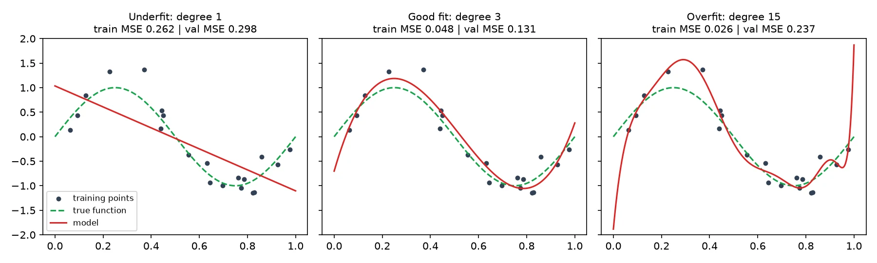
Part 1, one split. The degree-1 line has a training MSE of 0.262 and a validation MSE of 0.298. Both are about three times the 0.090 noise floor and only 0.036 apart: underfitting. The degree-15 model has the lowest training MSE (0.026) and a validation MSE of 0.237, a gap of 0.212: overfitting. Degree 3 has the lowest validation MSE (0.131). With only 20 points, even its training MSE (0.048) sits below the noise floor, a reminder that training error is always optimistic.
Part 2, complexity. Training MSE never goes up as the degree rises, from 0.262 at degree 1 to 0.026 at degree 15. Validation MSE drops to 0.131 at degree 3, then jumps around between 0.143 and 0.338. That erratic validation error is itself a sign of overfitting: with 20 points, the high-degree fits change a lot from one setting to the next.
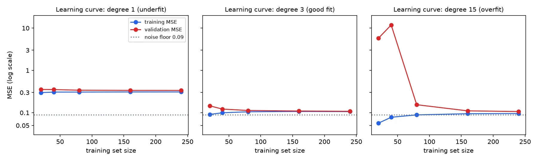
Part 3, learning curves. This is the part that tells you what to do next.
- Degree 1: validation MSE only moves from 0.354 to 0.336 as the training set grows from 20 to 240 points, and training MSE settles around 0.310. Both plateau far above 0.090. Twelve times more data barely helped, which is the underfitting signature.
- Degree 3: the gap closes from 0.054 to 0.002 and validation MSE reaches 0.108, close to the noise floor.
- Degree 15: with 20 or 40 points, validation MSE averages 5.766 and 11.852. The median and worst columns explain the odd jump: at 40 points the median split scored 0.192, but one split scored 230.569. An overfit model can do very badly on some data, which an average hides. By 240 points the gap is down to 0.011 and validation MSE is 0.107, a near tie with degree 3 (0.108). More data was enough to fix this overfit.
Part 4, regularization. Cross-validation on the 20 training points picked $\alpha = 0.032$. Validation MSE fell from 0.237 (no penalty) to 0.115, lower than the best plain polynomial (0.131), and the largest coefficient shrank from 1,391 to 2.32. Push $\alpha$ to 10 and training MSE climbs to 0.194: too much regularization creates underfitting.
Part 5, epochs. At epoch 10 both errors are still high (0.123 and 0.176). Validation MSE is lowest at epoch 25 (0.105). After that, training MSE keeps falling, to 0.003 by epoch 3,000, while validation MSE rises to 0.177. Stopping at the best epoch would keep the 0.105 model.
The two optional figures the script saves with --plot show parts 1 and 3: the three fits over the training points, and the three learning curves on a log scale.
How to fix underfitting
- Add features that carry real signal. Domain-driven features, interactions and transformations (such as polynomial terms or logs) often matter more than the model choice. Feature engineering is the most common fix for tabular data.
- Use a more flexible model. Move from a linear model to polynomial terms, tree ensembles or a larger network.
- Reduce regularization. Part 4 shows a penalty that is too strong pushes a flexible model into underfitting.
- Train longer or tune the optimizer if the loss is still falling when training stops, as at epoch 10 in Part 5.
- Don’t expect more rows to help. Part 3’s degree-1 curve shows why.
How to fix overfitting
Add L2 or L1 regularization
Regularization adds a penalty on large weights to the cost the model minimizes. A common way to write the L2-regularized (ridge) cost for linear regression is:
$$J(\theta) = \frac{1}{2m} \sum_{i=1}^{m} \left( h_{\theta}(x^{(i)}) – y^{(i)} \right)^2 + \frac{\lambda}{2m} \sum_{j=1}^{n} \theta_{j}^{2}$$
- $J(\theta)$ is the regularized training cost the optimizer minimizes.
- The first term is the usual squared error over the $m$ training examples. The $\frac{1}{2}$ is a convention that tidies the derivative; it doesn’t change which $\theta$ wins.
- $\lambda \ge 0$ is the regularization strength. At $\lambda = 0$ you get plain least squares; larger values push the weights toward zero.
- $\theta_{j}$ for $j = 1, \dots, n$ are the $n$ feature weights. The intercept $\theta_{0}$ is usually not penalized, which is why the sum starts at $j = 1$.
- $\theta_{j}^{2}$ makes large weights expensive, so the model prefers smoother functions that can’t chase every noisy point.
Multiply $J(\theta)$ by $2m$ and you get $\sum_{i} ( h_{\theta}(x^{(i)}) – y^{(i)} )^2 + \lambda \sum_{j} \theta_{j}^{2}$, which is exactly the objective scikit-learn’s Ridge minimizes, with its alpha playing the role of $\lambda$. Because the penalty depends on the size of each weight, scale the features first, as the demo’s StandardScaler does.
L1 (lasso) swaps the squared weights for absolute values, for example $\frac{\lambda}{m} \sum_{j=1}^{n} \lvert \theta_{j} \rvert$ (scaling conventions vary between libraries). L1 can set some weights exactly to zero, so it also selects features. Elastic net mixes both. The linear regression expert tutorial covers ridge, lasso and elastic net in more depth.
Pick $\lambda$ on validation data or with cross-validation, never on the test set.
Get more data, or augment it
Part 3 shows the effect directly: the same degree-15 model went from a validation MSE of 5.766 at 20 points to 0.107 at 240. When more labeled data isn’t available, data augmentation (flips and crops for images, for example) can help, as long as the transformed examples are realistic.
Stop training early
Track validation loss during training and keep the weights from the best epoch. Most frameworks support this directly: scikit-learn’s MLPRegressor has early_stopping=True with validation_fraction and n_iter_no_change, and Keras has an EarlyStopping callback with a patience setting. Google’s crash course describes early stopping as a form of regularization.
Use a simpler model or fewer features
Lower the polynomial degree, limit tree depth, use fewer layers or units, or drop features that add noise rather than signal. Feature selection and L1 regularization both reduce the number of things the model can memorize.
Add dropout to neural networks
Dropout randomly switches off a fraction of units on each training step, so the network can’t rely on any single unit. It was introduced as a way to reduce overfitting in Srivastava et al. (2014). It applies only during training; at prediction time all units are used.
Use cross-validation to tune, not a single lucky split
With small datasets, one validation split can mislead you; Part 3’s worst-case column shows how much results vary between splits. k-fold cross-validation averages over several splits, which makes choices like $\lambda$, tree depth or the number of epochs more reliable. Cross-validation doesn’t fix overfitting by itself; it helps you see it and choose the fix.
The same logic applies to large language models: fine-tuning on a small dataset can overfit too, which is one of the trade-offs covered in RAG vs fine-tuning.
A step-by-step diagnosis checklist
- Split the data first: training, validation (or cross-validation folds) and a test set you touch once at the end.
- Get a baseline, such as predicting the mean or using a simple linear model, so “high error” has a meaning.
- Compute training and validation error and the gap between them.
- Plot a learning curve against training-set size to see whether more data would help.
- Plot a validation curve against your main complexity setting, and a loss curve per epoch if the model trains iteratively.
- Apply one fix at a time from the matching list above and measure again.
- Check the test set once with the final model.
Common mistakes
- Choosing the model with the best training score. Part 2 shows training error never rising up to degree 15, while validation error was lowest at degree 3.
- Adding data to an underfit model. It rarely helps. Change the model or the features.
- Tuning on the test set. After that, the test score no longer measures generalization. Use validation data or cross-validation for tuning.
- Trusting one validation split on a small dataset. Results swing between splits; use cross-validation and look at the spread, not just the mean.
- Regularizing unscaled features. The penalty then hits features measured in large units harder than others. Standardize first.
- Letting preprocessing leak. Fitting a scaler or feature selector on the full dataset before splitting lets validation data influence training. Put preprocessing inside a pipeline, as the demo does.
- Calling every train/validation gap overfitting. If validation data comes from a different distribution than training data, the gap may be data shift, and model fixes won’t close it.
Frequently asked questions
What is the difference between overfitting and underfitting?
Underfitting means the model is too simple to capture the real pattern, so training and validation error are both high. Overfitting means the model has learned noise in the training data, so training error is low but validation error is much higher. One fails on everything; the other fails only on new data.
How do I know if my model is overfitting?
Compare training and validation error. If training error is low and validation error is much higher, the model is overfitting. A learning curve confirms it: a wide gap between the two curves that narrows as you add training data. In neural networks, validation loss that starts rising while training loss keeps falling is the same signal.
What does underfitting look like on a learning curve?
Both curves flatten out early at a high error, close to each other, and adding more training data barely moves them. That plateau tells you the model lacks the capacity or the features to learn the pattern, so more rows of the same data will not fix it.
Does more data fix overfitting?
Often, yes. More data makes it harder for a flexible model to memorize noise, so the gap between training and validation error shrinks. It does little for underfitting. If you can’t get more data, use regularization, a simpler model, early stopping or data augmentation.
How does regularization prevent overfitting?
Regularization adds a penalty for large model weights to the training cost. L2 (ridge) shrinks all weights toward zero, and L1 (lasso) can set some exactly to zero. Smaller weights give smoother functions that follow less noise. The strength, often called lambda or alpha, should be tuned on validation data or with cross-validation.
What is early stopping in machine learning?
Early stopping ends training when validation error stops improving, then keeps the weights from the best epoch. It works because a model trained for too long starts to fit noise: training loss keeps falling while validation loss turns upward. Most frameworks offer it as a setting or callback with a patience parameter.
Sources
All checked on October 21, 2026.
- scikit-learn: Underfitting vs. Overfitting example
- scikit-learn: Validation curves: plotting scores to evaluate models (validation curves and learning curves)
- scikit-learn:
learning_curveAPI reference and Plotting learning curves example - scikit-learn:
RidgeAPI reference (objective function) and Linear models: ridge and lasso - scikit-learn: Cross-validation: evaluating estimator performance
- scikit-learn:
MLPRegressorAPI reference (early_stopping, partial_fit) - Google Machine Learning Crash Course: Overfitting, Model complexity, L2 regularization and early stopping, Interpreting loss curves
- Srivastava, Hinton, Krizhevsky, Sutskever and Salakhutdinov: Dropout: A Simple Way to Prevent Neural Networks from Overfitting, JMLR 15 (2014)
- Keras: EarlyStopping callback
- Hastie, Tibshirani and Friedman: The Elements of Statistical Learning (model assessment and selection, regularization)
Learn machine learning with guided practice. For more guides like this, browse the machine learning tutorials hub, starting with bias vs variance. For live, instructor-led classes with hands-on Python labs, see AI and machine learning training, or the full list of training courses. If you are in the United States, see online AWS and AI/ML training in the USA.
Newsletter
Enjoyed this post?
Get new posts, AI/ML tutorials, AWS batch dates and Oracle tips by email. No spam, unsubscribe anytime.